STAT2008/STAT2014/STAT4038/STAT6014/STAT6038 REGRESSION MODELLING Assignment 1

RESEARCH SCHOOL OF FINANCE, ACTUARIAL STUDIES AND STATISTICS

REGRESSION MODELLING

STAT2008/STAT2014/STAT4038/STAT6014/STAT6038

Assignment 1 (Total Marks: 50)

Submit by 5pm on Tuesday 20 Apr 2021

INSTRUCTIONS:

• This assignment is worth 15% of your overall marks for this course and redeemable.

• You must write up your solutions to this assignment by yourself. If you copy someone else’s work or allow your work to be copied, you will receive a mark of zero for the assignment and risk very severe academic consequences.

• Your report should be submitted to Turnitin on Wattle as a single pdf document (less than 50MB) including the following:

1. The assignment cover sheet (available to download from Wattle).

2. Your assignment (no more than 10 pages).

3. An appendix including all the R commands you used (no page limit).

• Assignments should be typed. Your assignment may include some carefully edited R output (e.g., graphs, tables) and appropriate discussion of these results, as well as some selected R commands. Please be selective about what you present and only include as many pages and as much R output as necessary to justify your solution. Clearly label each part of your assignment and appendix with the question number and the part of the question that it refers to.

• Unless otherwise advised, use a significance level of 5%.

• Round numeric answers to 4 decimal places (e.g., 0.0012).

• Marks will be deducted if these instructions are not strictly adhered to, especially when the total report is of an unreasonable length, i.e., more than 10 pages including graphs and tables. The appendix and the cover sheet are in addition to the above page limit; but the appendix will generally not be marked, only checked if there is some question about what you have actually done.

• Name your report “Course code_Uid”, e.g., “STAT2008_u1234567”.

• Try to submit your assignment at least 15 mins before the deadline in case something unexpected happens, for instance internet issue.

• Late submissions will NOT be accepted. Extensions will usually be granted on medical or compassionate grounds on production of appropriate evidence, but must have lecturer’s permission at least 24 hours before the deadline.

Question 1   [13 Marks]

As we know, b0 and b1 are the least squares estimators of the unknown parameters β0 and β1 of simply linear regression model, respectively. In this question, we will study the correlation between b0 and b1 both from theory and numerical simulations. The simulation codes are provided as follows:

# Set your Uni ID number as the seed of random number generator.

# For example, if your Uni ID is u1234567, then use

# set.seed(1234567)

x <- 1:10

n <- length(x)

estimates <- matrix(NA, 1000, 2)

names(estimates) <- c("b0","b1")

for(r in 1:1000) {

y <- 1 + 2*x + rnorm(n,0,2)

estimates[r,] <- lm(y~x)$coefficients

}

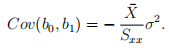
(a) [4 marks] Show the covariance of b0 and b1:

Note that you cannot use the matrix approach introduced in week 6.

(b) [4 marks] Write down the true model and the distribution of the error terms used in the simulation. Based on this model, calculate the values of the theoretical covariance and correlation of b0 and b1.

(c) [2 marks] First set your Uni ID number as the seed of random number generator, e.g., if your Uni ID is u1234567, run set.seed(1234567). Then run the simulation. Make a scatterplot of b1 against b0 based on the simulation output. Do these estimates appear to be correlated?

(d) [3 marks] Following part (c), calculate the values of the empirical covariance and correlation of b0 and b1. Comparing the results with part (b), what do you notice?

Question 2   [37 Marks]

Data file “mammal.csv” (available to download from Wattle) contains the average mass (Mass) in kg, metabolic rate (Metab) kJ per day and average lifespan (Life) in years for 95 species for mammals. It has been suggested that metabolic rate is one of the best single predictor of species lifespan.

(a) [3 marks] Make a scatterplot of Life against Metab and visually check if there are any high leverage observations. What are the names and species of these mammals?

(b) [2 marks] Make a comment on the relationship between Life and Metab for the majority of observations. You may need to adjust the x and y coordinates ranges.

(c) [5 marks] Apply natural log transformation to Metab. Then fit a simple linear regression model by regressing Life on transformed Metab. Provide the fitted results. Then conduct model diagnostics. Provide the appropriate plots and discuss your findings regarding model assumptions and unusual observations.

(d) [4 marks] Following the model in part (c), experiment with applying natural log transformation and square root transformation to the response variable. Select a best model with the help of scatterplots and sample correlations. Write down the mathematical form of your selected regression model.

(e) [4 marks] Following your selected model in part (d), fit a simple linear regression model. Write down the fitted model by mathematical equation. Conduct model diagnostic, provide the appropriate plots and discuss related results.

(f) [3 marks] Interpret the estimated slope of the fitted model in part (e). Obtain a 95% confidence interval for the slope parameter.

(g) [5 marks] Using ANOVA approach to test whether the model in part (e) is signifi- cant. You need to write down the hypotheses, provide the ANOVA table. What is the test statistic, rejection region or p-value, and your conclusion associated with this test?

(h) [4 marks] With the model in part (e), find a 90% prediction interval for the lifespan in years of a mammal with the metabolic rate 8000 kJ per day. Interpret this interval.

(i) [7 marks] Kleiber’s law states that on average the metabolic rate of an animal species is proportional to its mass raised to the power of 3/4. Propose a simple linear regression model and appropriate hypotheses to check the adequacy of this theory and explain why. Using this dataset, fit the model and provide the fitted results. Then test your proposed hypotheses. What’s your conclusion?