Numerical Methods for Finance Individual Project

Numerical Methods for Finance

Individual Project

This is a individual project that is worth 15% of the overall grade. All Python code should be taken from the slides and adjusted accordingly. Code taken from other sources will not be accepted.

1. Consider an American put option written on a non-dividend paying stock. Assume the stock price follows geometric Brownian motion with an initial stock price of S = 100 and with an instantaneous volatility of σ = 30%. Assume the continuously compounded interest rate is constant at r = 5%, and let the option strike price be K = 105 with a time-to-maturity of 6 months.

(a) Adjust the Python code below (see last page of this assignment) to price this Ameri-can put option using binomial trees.

(b) Adjust the code in the slides to price this American put option using the explicit finite difference method.

(c) Adjust the code in the slides to price this American put option using the implicit finite difference method. Do this with the following approaches: (i) an LU decomposition linear solver as per the code in the slides (ii) a Gauss-Seidel iterative solver that re-places the American option price (as soon as it is updated) with the maximum of the early exercise value or the option continuation value and (iii) a Gauss-Seidel succes-sive over-relaxation solver (in SOR you should experiment with the over-relaxation parameter ω to find the right value that speeds up convergence).

(d) Compare and contrast the above American put option prices at different discretisation levels for both the stock price and time-to-maturity. Analyse and comment on your results.

2. (a) Price a down-and-out European put barrier option with specifications as in Section 1 above along with a knock-out barrier at SB = 70 such that the European put option becomes worthless if the barrier is hit from above. Price this option using (i) a bino-mial tree, (ii) an explicit finite difference method and (iii) the Crank-Nicolson finite difference method combined with a linear system solver of your choice. Compare and contrast the price of the European put barrier option to a plain vanilla European put option.

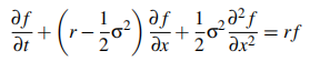
3. The partial differential equation (PDE) for an option price f = f(x,t) where the option price is expressed as a function of the log stock price, x = lnS, and time t is given as follows:

The grid for the log stock price is given as xvec = [xmin, xmin +δx, xmin +2δx,..., xmax — δx, xmax] however, we cannot set Smin = 0 as this means xmin = ln(0) = = — ∞, so we set . Similarly, set . Set L = 3 initially but when the code is up and running you can experiment with this value to obtain a value for L that is suitable.

(a) Derive the coefficients on the explicit finite difference algorithm by discretising the above PDE and solving for fi, j-1 in terms of fi+1, j, fi, j and fii-1, j.

(b) Derive the coefficients on the implicit finite difference algorithm by discretising the above PDE and solving for fi+1, j-1, fi, j-1 and fi-1, j-1 in terms of fi, j.

(c) Price the same American put option as before but now using the log stock price as the stochastic state variable (as opposed to the stock price) using the following methods: (i) the explicit finite difference method, and (ii) the implicit finite difference method with a Gauss-Seidel linear solver.

(d) Compare and contrast the output in Section 3 to the output from Section 1.

Complete the above exercises in a Jupyter Notebook. To submit your file select “file\print pre-view” from the top left corner of your Jupyter Notebook and in the print preview browser page select “Print to PDF” from the top right corner (the three vertical dots on Chrome), save the PDF file to your computer and submit the PDF file to the Assessment tab on the module’s Brightspace page by 6pm Monday 29th of March. In your Jupyter Notebook you should include a short introduction, method, results and conclusions detailing your analysis. Write these sections in Markdown cells rather than Code cells. Provide plots of results where appropriate, including axis legends and plot titles.

Please start your code with the code examples in the slides (or the example given below). If you are coding an example that is not in the slides please use the notation from the slides along with the existing code in the slides and adjust as required for the task at hand. Code taken from the internet or any other sources will not be accepted.

The code on the next page defines a function to price a European put or call option on a non-dividend paying stock that follows geometric Brownian motion using the binomial option pricing model. The usual notation applies with S denoting the stock price, K the strike price, r the riskless (continuously compounded) rate, T the time-to-maturity and σ the volatility of the stock price process.

import numpy as np

from numba import jit

@jit

def binomialEuropeanOption(S, K, r, T, sigma, n=100, option='call'):

deltaT=T/n

u=np.exp(sigma * np.sqrt(deltaT))

d=1.0 / u

a = np.exp(r*deltaT)

q=(a-d) / (u-d)

Sv = np.zeros((n,n))

V= np.zeros((n,n))

# Build stock price matrix forward

for j in range(n):

for i in range(j+1):

Sv[i,j] = S* u**i * d**(j-i)

if option == 'call':

CorP = 1

elif option == 'put':

CorP = -1

V[:,-1] = np.maximum((Sv[:,-1]-K)*CorP,0)

# Price option with backward induction

for j in reversed(range(n-1)):

for i in range(j+1):

V[i,j]=np.exp(-r*deltaT)*(q*V[i+1,j+1]+(1.0-q)*V[i,j+1])

return V[0,0]