ENGF0003 Modelling Populations

Hello, dear friend, you can consult us at any time if you have any questions, add WeChat: daixieit

Modelling Populations

ENGF0003 LSA Coursework

Information

Release Date: Friday 25th July 2025

Submission Deadline: Friday 22nd August 2025

Estimated Coursework Return: Four weeks after submission

Topics Covered: Topics 1 - 5

Expected Time on Task: 12 hours

• Read this document thoroughly before starting your work. Use the Moodle forum to ask any questions you might have, or to check answers given to your colleagues. No questions will be answered on the week before the coursework’s deadline unless you have a SORA.

• Do not write down your name, student number, or any information that might help identify you in any part of the coursework.

• Do not copy and paste the coursework brief into your submission – Rewrite information where necessary for the sake of your argument.

• Type your answers in Microsoft Word or any text editor, insert relevant graphs or figures, and describe any figures or tables in your document.

• All figures and tables must be labelled, with their axes showing relevant parameters and units. Number the main equations throughout your work for ease of reference.

• Submit a single PDF document with font size 12 and 1.5 line spacing. Give preference to simple and familiar fonts such as Arial, Helvetica, Calibri, Tahoma, Georgia, and Verdana. Name your file ENGF0003CW.

This coursework counts towards 20% of your final ENGF0003 grade.

Problem Context

The human population on Earth has been increasing over the last 12000 years. This increase has intensified in the last few hundred years, where we have seen a 13-fold increase since 1700 (Figure 1). There are many reasons for such growth including developments in sanitation, food production, medicine and housing to name only a few, but it is not known whether this growth will continue and for how long.

One controversial topic in the debate is the maximum human population that Earth can sustain, known as the carrying capacity of Earth. Research in this field estimates a wide range of values ranging from just under 2 billion people to 1 trillion people [1]. With a current world population exceeding 8 billion people, it is clear that we must engineer ways of living that are socially equitable and do not deplete resources for future generations.

The rising population of Earth has been linked to a number of global problems such as climate change [2, 3], increased risk of pandemics [4] and resource depletion [5]; however, there are also positive outcomes associated with population increase such as increased scientific and industrial innovation [6] and increased economic growth [6] which can lead to overall increased welfare of the population.

The UNESCO maintains that “Engineers have played a key role in transforming the world through invention and the development of new technologies, which has had a significant impact on economic growth and quality of life”, but now calls engineers to consider how to use resources in a way that does not compromise the environment or exacerbates social inequality. According to UNESCO, we must become engineers that are empowered to make “informed decisions in favour of environmental integrity, economic viability and a just society for present and future generations” from as early as our training at university [7].

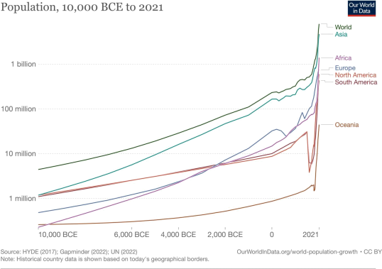
Figure 1. World population from 10,000 BCE to 2021. Source: https://ourworldindata.org/population-growth

Forecasting the human population on Earth then becomes a sustainability challenge. How many humans can the natural resources of the planet support, and how many humans can live in the Planet sustainably? This question is complex because it involves conflicting interests between society, the environment and the economy.

In this coursework, you will explore the mathematics used to model and predict population growth over the years and give your own opinion about their suitability to explain this phenomenon. We are also interested in hearing your opinion about the dangers and benefits of using mathematical models to analyse and predict population growth on planet Earth.

Mathematical Models

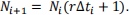
The discrete Malthusian model states that a population grows over time as

                 (1)

In this equation, Ni represents the number of individuals at a certain time ti. If these individuals grow at a rate r during a time interval  then the number of individuals at ti+1 is given by Ni+1, as shown in Equation 1. Click here to watch a video demonstration of this model by Khan Academy.

When rearranged in differential form, this model is given by Equation 2:

                (2)

One of the main limitations of the Malthusian model is that it does not account for a growth rate that is a function of the size of the population. The Logistic model given in Equation 3 addresses this limitation by including the term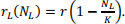 

In the Logistic model, K is the carrying capacity of the environment where the population grows,

and NL is the population predicted by the logistic model:

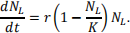             (3)

Deliverables

The data attached to this brief contains time-series measurements of the population in planet earth obtained from the “Our World in Data” project. The entries are separated by low- and high-income countries as well as for the whole world.

1. Summarise and Communicate the Data

20 MARKS – 2 PAGE LIMIT

Your task is to summarise and describe the dataset attached to this brief and communicate the main patterns in the data in a concise, accurate and accessible way.

1.1. Produce one table summarising key metrics and statistics in the dataset.

1.2. Provide one short paragraph (300 words or less) justifying why you have chosen to summarise the data in the way you did.

1.3. Explain the main trends and patterns you can take from the numerical summary of the data.

2. Model and Evaluate Linear Behaviours in the Data

30 MARKS – 2 PAGE LIMIT

Your task is to create data-driven models of the data. Calculate a linear regression of the population size N as a function of time t in each of the groups: low-income, high-income, and whole world.

2.1. Explain what the coefficients of the linear regression mean and evaluate the quality of the regressions by calculating, contrasting and comparing the coefficient of determination R2 for each model.

2.2. Produce figures containing scatterplots of the population with respect to time for each of the groups: low-income, high-income, and whole world. Plot your linear regressions over the scatterplots.

2.3. Using your linear regression results, as well as your plots, describe population growth in the three groups contained in the dataset.

3. Model and Evaluate Non-Linear Behaviours in the Data

30 MARKS – 2 PAGE LIMIT

3.1. Apply your knowledge of differential equations to obtain a function N(τ) modelling population growth according to the Malthusian model from Equation 2, as well as NL(τ) for the Logistic model from Equation 3, where τ represents time in both results.

3.2. Use your solutions in 3.1. to adapt the template code provided in the next page to estimate the values of r and K from the data for the Logistic model, and the value of r for the Malthusian model. Remember to provide group-specific estimates: for low-income countries, high-income countries, and the whole world.

3.3. Contrast and compare the accuracy of the predictions of the linear regressions from Deliverable 2 against the accuracy of the fitted non-linear models N(τ) and NL(τ) in 3.2. What have you learned from this?

Template code:

4. Reflection of Learning

20 MARKS – 1 PAGE LIMIT

Write a conclusions section for your coursework. Write paragraphs or use bullet points summarising the main ideas and take-aways from each section in terms of:

• What you have learned while doing each question. Contrast and compare your knowledge, skills and attitudes before your studies at UCL and after completing this Coursework.

• What are the implications of your results for the environment, society, and the economy. Provide a reasoning of what is important to you in analysing populational growth problems. Make a statement about how engineering students should approach problems involving mathematics and society.

References