关键词 > PHYS5033
PHYS5033 Environmental Footprints and IO Analysis Week 4
发布时间:2025-08-14
Hello, dear friend, you can consult us at any time if you have any questions, add WeChat: daixieit
PHYS5033
Environmental Footprints and IO Analysis
Reading Material
Week 4
Week 4 Leontief,s methodology and the fundamental input-output equation
Once data has been collated into an input-output table, Leontief,s methodology can be implemented. There are a number of assumptions made with this methodology, which include (Dixon, 1996; Kitzes, 2013; Miller & Blair, 2009):
• Industries use the goods and services of other industries to produce their own goods or services, so the outputs of one industry are the inputs of another
• Transactions are accounted for in monetary terms
• There is a linear relationship between demand for inputs and outputs 一 if demand increases the output increases proportionately to meet the increased demand
Leontief,s methodology relies on two key matrices 一 the direct requirements matrix (A) and the total requirements matrix (L). The steps taken to derive these two matrices from the T, v, and Y matrices provided in the input-output table are outlined below.
Calculate the total output (x) of the input-output table
This was discussed in detail in week 2 and provides a column vector of size (m x 1) where m represents the number of sectors in the input-output table. Total output is calculated using the following equation:

Calculate the direct requirements matrix (A)
The direct requirements matrix (A), also known as the direct coefficients matrix, provides information on the direct inputs required from each sector to produce $1 of output for a given sector. Mathematically this can be calculated by dividing the values in T by the total output x for a sector, which can be expressed as:
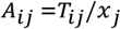
where i and i represent the rows and columns in T respectively.
However, because we are dealing with matrices, this calculation is not as simple as it might appear. Once again, we need to consider the sizes of the matrices being used and note that x will always be a (m x 1) vector, which means that it cannot be divided into T, which will be a (m x m) matrix.
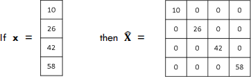
To enable us to carry out these calculations, we rely on matrix diagonalisation and inversion, which were introduced in the reading material for week 2. A square matrix which contains zero values in all elements above and below the main diagonal is known as a diagonal matrix. Converting a (m x 1) matrix x to a diagonal matrix involves creating a (m x m) matrix with all zero values, and then placing each element of x on the diagonal such that x1 is placed in the element in the first row and first column, x2 is placed in the element in the second row and second column, and so on until xm is placed in the element in the mth row and mth column. The annotation used to indicate diagonalisation of a matrix is ![]() .
.
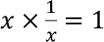
The inverse of a square matrix can be calculated by considering that the Identity matrix (I) has similar properties to the number one (1) in non-matrix mathematics. Just as any number multiplied by its inverse will have a value of one:
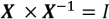
any matrix (X) multiplied by its inverse (X-1) will return the Identity matrix (I), with dimensions equal to the original matrix:
We use this property to calculate the inverse of X(^), and thus create a matrix which can be multiplied by T to calculate the direct requirements matrix (A):

Since T is a component of x, the values of each of the elements in A must be less than or equal to 1, or expressed mathematically:

The steps required to calculate A using Excel are included in Figures 4.1 to 4.3.
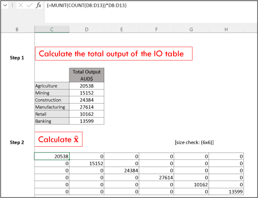
Figure 4.1: Excel screenshot when converting the total output vector x to a diagonal matrix x(^).
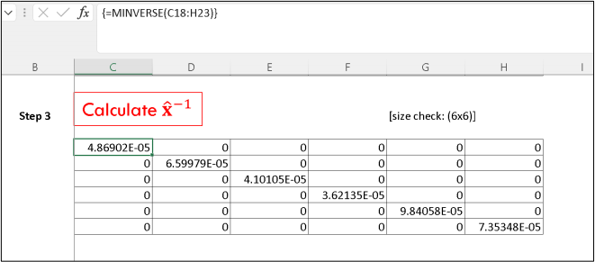
Figure 4.2: Excel screenshot when using MINVERSE to calculate the inverse of x(^).
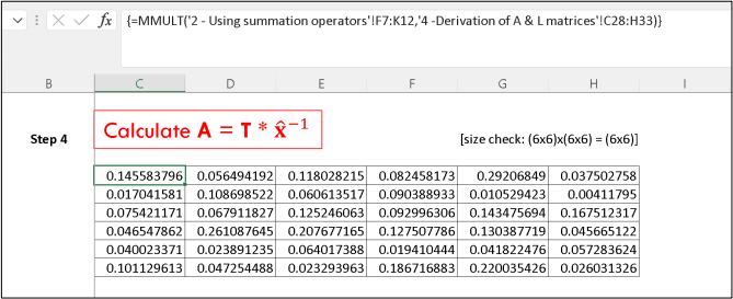
Figure 4.3: Excel screenshot when using MMULT to calculate A = T * x(^) -1.
