Marketing

Comprehensive Problem Set (CPS) [Optional]

Block 1:    Answer 2 of the following 3 questions. 50 points per problem.

1.   A Monopsony is the lesser-known sibling of a Monopoly.    While a Monopoly is a market with    only one seller of a good, a Monopsony is a market with only one buyer of a good.    This leads to its own kind of market failure.

[Some context if you are interested: Monopsony comes up most frequently in labor markets.    As an interesting example, professional

sports leagues have many characteristics of Monopsonies.    The NFL is the pretty much the only elite league for professional football.      If you want to play pro football at a high level, the NFL is the only entity that will buy your services.    This gives the NFL market power over players, and probably limits the amount the league pays for player salaries, through features like “salary caps” and other restrictions. [As an aside, I speculate that, since European soccer has many elite professional leagues, this probably leads to higher player salaries in    soccer.    Kylian Mbappe, for example, recently had a contract that paid $ 121 million per year over two years (with signing bonus) for

PSG.    Cristiano Ronaldo supposedly is being paid $220 million to play in the Saudi pro league, though his particular high salary is probably due to other factors.    Meanwhile, Dak Prescott in the NFL is the highest paid player at “only” $60 million per year,]

A company/factory town would be another example of a Monopsony.    If there is only one significant employer buying labor in a local area, that employer will have a unique type of market power over its employees. Fewer jobs with lower  salaries will be the result in a Monopsony, as you will discover.]

The analysis for market failure with a Monopsony is similar to that of a Monopoly, with one key  difference.    Your goal in this problem, if you attempt it, is to figure out how that works.    If you study the notes from our class on Monopoly, and try to apply our method to the Monopsony case, that will hopefully provide some hints on how to analyze this situation.    Now for the problem:

A market for a good is characterized as a Monopsony.     There are many sellers and a single buyer of the good, the “Monopsonist”.

The Supply curve is: PS(Q)= 100+ 1.8Q

The Marginal Benefit to the Monopsonist from buying the good is PB(Q)= 2000-1.4Q

a.)  What is the efficient quantity and price of the good?

b.)  What is the equilibrium quantity and price of the good?

c.)  What is the Marginal Benefit to the Monopsonist at the equilibrium?

d.)  What is the deadweight loss created by the Monopsonist?

2.   Beekeeping for the purpose of making honey provides external benefits to farmers located near the beehives, as bees pollinate their plants and improve crop yields.    Bees also produce negative externalities.    Being stung by bees is unpleasant.    The more bees in a certain area, the more likely it is that people will be stung. In addition to hurting, some people have alergic reactions to stings and thus it can clearly be costly.    Suppose we have the following situation.

Marginal Benefit to Honey Consumers from an additional beehive: MPB=5000-75Q

Marginal External Benefit to neighboring farmers from an additional beehive: MEB=1000+.2Q

Marginal Cost to Honey Producers of an additional beehive: MPC=500+5Q

Marginal External Cost to neighbors from additional beehives: MEC=0+. 1Q

a.)  Find the market equilibrium Quantity and Price of hives.

b.)  What is the MSB  at the Market equilibrium? MSC?

c.)  What is the socially optimal (Efficient) level for this society?

d.)  What is the Deadweight loss at the Market equilibrium?

e.)  What is the tax/subsidy that will lead to a new Market equilibrium at the Optimal quantity?

3.   Suppose the government wishes to reduce the amount of methane gas, a waste product created from refining petroleum.    Suppose the marginal benefit to society from reducing (abating) methane from the current levels is constant at $6000 per gigaton.

Abatement levels will be on the x-axis and Costs on the y-axis.

Assume that there are four producers, named 1, 2,.3, 4.

The marginal abatement costs are:

Producer 1: MAC, 1 =.3A1.

Producer 2: MAC,2= .5A2.

Producer 3: MAC,3= .6A3

Producer 4: MAC,4= (1/3)A4

The total amount that is ultimately abated is A=A1+A2 +A3+A4

a.)  The Marginal Abatement Cost (MAC) for the whole market is the horizontal sum of the

individual producers’ marginal abatement costs.    What is the market-wide MAC as a function of A? [Note, the coefficient on producer 4 is 1/3, which will give a beautiful clean answer in the end.    If you round 1/3 to .333 or something be aware that it will be slightly off, but you can probably guess what the number is suppose to be.]

b.)  Given the answer to 1, what is the socially optimal level of methane abatement?

Prior to any abatement, Producer 1 produced 9000 gigatons of methane, Producer 2 produced 10000 gigatons, Producer 3 12000 gigatons,    Producer 4 produced 11000 gigatons.    The total methane is thus 42000 gigatons.

c.)  The government wishes to use permits to achieve the optimal abatement.    Each permit will allow the owner to produce 1 gigaton of methane. How many permits must the government issue to achieve the optimal abatement level?

d.)  If the permits were not tradeable, how much must each firm abate, and what are the

Marginal abatement costs for each firm when they reduce their pollution to the permitted level?

e.)  If the firms can buy/sell their permits with one another, how much abatement does each firm do in the equilibrium?

Block 2: Answer 2 of the following 3 problems.

1.  Congestion Pricing

This problem models market inefficiencies related to a congestible public good: a road.    We did this model one day in class.    You should refer to that work for guidance. I’ve made one adjustment in the effect of traffic on speed.

The ingredients of the problem are:

N- the number of cars on the road.

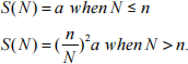
n=2000 the threshold number of cars.    Below this threshold, cars do not lead to traffic slowdowns. N above n will lead to a slowdown in traffic speeed, as described in the formula below.

a=55 the speed of traffic, in MPH, withen N

S(N)-the speed, in MPH of a car as function ofN.

b= 50, opportunity cost of an hour spent in car.

a)   Write down the function T(N), which is the time to travel one mile.

b)   The ATC is the average opportunity cost of driving one mile.    Write the the ATC as a function of N.

The ATC is each driver’s perception of their marginal cost of driving one mile.     So we can also think ofit as the MPC.

c)   Calculate the Total Cost function (TC(N)) to society of having N drivers on the road. [Hint: you’ll know you’re at least on track if you have N3  in your formula.]

d)   You can use Calculus and take the derivative of TC(N) wrt N to get the MSC function.    Doing the equivalent algebraically is pretty annoying (I assume it is, at least, as I haven’t done it).    But since Calculus is not required in this class, here’s the general result: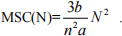

The MSB of driving is 10-.002N.

e)   What is the market equilibrium level of traffic, N*?

f)   What is the optimal level of traffic, N+?

g)   What is the toll on drivers that will deliver N+?

h)   Estimate the deadweight loss resulting from the inefficient level vs the optimal level.     [Because the change in speed is non-linear, this will not be triangle with straight sides     (one side will be a curve).    But it will look triangle-ish. Your estimate can assume that all the edges are straight.]

2.  Suppose a society contains two individuals.    Joe, who smokes, and Tanya, who does not.     They each have the same utility function U(C)=ln(C).    If they are healthy, they will each get to consume their income of $ 15,000.    If they need medical attention, they will have to spend $ 10,000, leaving them $5,000 for conumption.    Smokers have a 12% chance of needing medical attention, and nonsmokers have a 2% chance.

An insurance company is willing to insure Joe and Tanya.     The twist here is that the insurance  company offers two different kinds ofpolicies.    One policy is called the “low deductible,” (L)  for which the insurance company will pay any medical costs over $3,000.     The other is a “high deductible,” (H) for which the insurance company will pay any medical costs over $8000.

a.   What is the actuarially fair premium for each type ofpolicy for Joe and Tanya?

b.   If the insurance company can determine who smokes and who does not, and they charge the actuarially fair prices to each, what policy will Joe select?    Tanya?

c.   Now, suppose that the insurer cannot determine who smokes and who doesn’t.    The

insurer sets prices for each product.    The price of L is $840 and the price of H is $40.

(Why did I choose these numbers?) What will Joe and Tanya choose to do?    Will adverse selection push Tanya out of the market?    [Hint: No.] Calculate the total expected utility    for our society under this outcome.

d.   What has happened here?    What does the second policy option accomplish?

e.   How does this outcome compare to the scenario we’ve done several times in class, where the government mandates both to get a full insurance plan (F), and the insurer charges the actuarially fair premium.

Block 3. Answer each of the following two questions.

1.   (50 points)We will imagine there being two markets for computers:    Home computers and

Business computers. The curves in these markets are linear, but I will not tell you what those     formulas are [you don’t need to know them to answer the questions].    However, I will tell you that at the equilibrium, the elasticity of demand for home computers is -2.5, the elasticity of demand for business computers is -.90, and the elasticity of supply for computers for both purposes is 1.

a.   (10) A per-unit tax of $200 is imposed on the suppliers of computers.    How much does the buyer price increase in each market?    You can and should do this without knowing  anything about the pre-tax equilibrium, if you use the elasticity formulas we covered in  lecture.

b.   (10) Suppose the untaxed market equilibrium price and quantity in the home computer

market are $850 and 10 million, respectively.    In the business market, the untaxed market equilibrium price and quantity are $ 1200 and 15 million, respectively. What is the total revenue from the tax?

c.   (10) What is the deadweight loss of the $200 tax?

d.   (10) Comment on the relative sizes ofthe DWL in the two markets.    Why are they different?

e.   (10) Imagine that you could tax the consumer and business markets separately.    That is, a different tax for each market.    Call these taxes th  and tb.What would these taxes be if   you wanted to generate the same level of revenue as part b, while minimizing the DWL? [To answer this part, it will greatly help if you use the formula for the marginal deadweight loss shown briefly in class.    Since the derivation of that required some     calculus and I don’t want you to have to derive it on your own, I’ll write it down right here for you to use: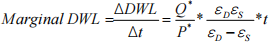

2.   (50 points) As described in lecture, the government can incentivize certain types of behaviors by allowing spending on those behaviors to be deducted from income.    One example of this is the  Mortgage Interest Tax Deduction (MITD). During a year, homeowners can subtract any spending on the interest payments from their mortgages from their income, lowering their income and their tax bill. In this problem we will explore this deduction in some detail, and how it may impact decisions on how much to borrow to purchase a house.

This problem requires a fair bit of set up.    I will walk you through it

Take a look at the following mortgage calculator linked below to help answer the following.

https://www.bankrate.com/calculators/mortgages/amortization-calculator.aspx

Suppose the value of a property is $500k (this number is not necessarily the loan amount, and will change for different parts of the problem), the interest rate is 5% (approximately the correct interest rate as of this writing), and the length of the loan (the “loan term”) is 30 years. Set the loan start date for January. Leave any other values at the default settings.    In the center of the  web page of the calculator, you can choose to view “Chart” or “Schedule.”    The Chart is nice,    but you’ll need the Schedule because that has the numbers.

Throughout the problem, the marginal tax rate for the borrower is 33%.

Assume the individual has $500k cash on hand, and any of this money that remains after taking     the mortgage/making mortgage payments is invested at the interest rate 3%.    The earnings ofthe investments can be taxed each year at the marginal rate. The value of the property also grows at rate 3% per year. This means that as the borrower repays the loan and starts building principal, the value of that principal goes up at the same rate as other investments.       However, the increased value of the property is not taxed, as the borrower doesn’t actually receive that increased value until or if they sell the property in the future. Finally, assume that the year’s mortgage payment is paid to the bank from cash on hand at the START of the year.     This turns  out to be important if we want to make comparisons. Homeowners are able to deduct the amount of interest paid on their mortgage when calculating taxes.

NOTE: There are 4 sets of calculations you will make before you are finished. I recommend you set up your answers in an excel spreadsheet. It will make the calculations much easier and faster.

i.    (10) Suppose there is no MITD, and the homeowner borrows the full value of the property ($500k). According to the mortgage calculator, for the first year:

a)   How large is the annual mortgage payment? How much interest has been paid on the mortgage?

b)   How much principal has been paid off by the borrower?

c)   The amount of the annual mortgage payment from part a) was paid at the beginning of the

year.    That reduces the cash available to invest.    How much cash gets invested? What is the pre-tax value of the cash investment at the end of the year?    How much tax is owed on this investment?    What is the after-tax value of the investment after one year?

d)   Add up the values of all the investor’s assets at the end of year one.       How has this value changed over the year?