CSYS5010: Introduction to Complex Systems

Hello, dear friend, you can consult us at any time if you have any questions, add WeChat: daixieit

Sand Dune Development and Environmental Factors

CSYS5010: Introduction to Complex Systems

June 2022

Aims and Design

The aim of the project was to develop a minimal model which can produce high-level sand dune features and can be used to make predictions of the landscape change.

There are variety of shapes and sizes of sand dunes found in nature, as depicted in figure 1.1.

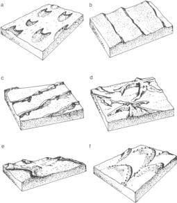
Figure 1.1: Classification of dunes (from Lancaster (1994) after McKee (1979)): a) barchans, b) crescentic ridges, c) linear, d) star, e) reversing, and f) parabolic

Generalised phase diagrams have been developed as early as Hack (1941), which depict the interplay between the environmental factors and the observed dune formations, however these are largely high-level as depicted in Figure 1.2.

The rules governing the behaviour of a dune system has no central actor how-ever multi-scale fractal patterns emerge. Dune systems also take on a variety of

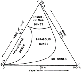
Figure 1.2: Phase Diagram from Hack (1941) showing the relationship between observed dune forms in Western Navajo Country and environmental conditions

different forms based on a range of environmental parameters. As such, an agent-based approach is particularly well suited to investigate the behaviour of such a system with many interdependent parts.

Aiming to discover the dynamics of the key environmental parameters on form-ing dunes, we have focused our work on the impact of the variable wind on the formation of different types of dunes which was not studied extensively previously. Additionally, we investigated the impact of vegetation and obstacles on sand dune development.

Implementation and Development Progress

In the following section, the modelling loop and sequence of extensions to de-veloping our final programs is described. For a full description of the code and explanation of the variables and functions, refer to Appendix B, and Appendix C and D for the developed code.

2.1 Minimal Model

We developed our model based on Werner (1995) model. In the Werner model, a dune field is modelled on a 2D grid with each cell consisting of a number of sand slabs, relating to the height of the sand for that area. Depending on the wind, a random slab is transported a number of cells and is deposited or continues being transported depending on the features of the target cell. Sand height on each patch is limited by the height of the surrounding patches to mimic avalanche conditions. The slab is likelier to be placed on a patch with existing sand rather than on bedrock. Additionally, patches to the leeward side of a dune ridge are in the dunes ‘shadow’, where sand is deposited immediately.

As an initial step, we modelled this behaviour with wind only coming from a single direction.

2.2 Variable Wind

Following the uniform wind, we used Netlogo’s patch-at-heading-and-distance function to control the wind speed and direction of deposited sand slabs.

2.3 Vegetation Extension

Following the Werner model Baas (2002) developed a rudimentary model to im-plement the effect of vegetation in sand dunes. Vegetation increases maximum angle of repose before toppling, and increases the probability of sand being cap-tured, while also growing according to some assumption of tolerance to erosion and burial.

2.4 Obstacle extension

Obstacles were modeled as an additional patch variable containing the height of the bedrock or obstacle at that location. The location of the obstacle can be interactively painted on the model view window at the height of the user’s choosing.

In this model, when each sand slab is being deposited, patches are sampled at specific locations along the path to determine whether there is a obstacle coming out of the ground. If the obstacle is taller than the surroundings by a certain amount, the sand particle is deposited on the previous patch before the obstacle. The obstacle also casts a wind ‘shadow’.

2.5 Mathematica Links

Analysis was mainly done through a Mathematica environment using the NetLogo-Mathematica link (Bakshy and Wilensky, 2007). Using this link, we were able to develop Mathematica code for efficient analysis and display of the sand elevation plots, and perform repeated simulations. Mathematica also facilitated the modi-fication of the wind each tick allowing for the implementation of bimodal wind distributions and real-life wind data.

Analysis of Results

Mathematica code for the following section is provided in Appendix D.

3.1 Parameter Search

3.1.1 Setup

Bimodal wind under variable mean sand heights was investigated to see the effect on emergent morphologies. This approach is similar to the one presented in Lü, Dong and Rozier (2018), where a variety of dune types were evolved based on the changing parameters of angle difference, strength ratio and sand supply.

A Mathematica script was produced to automate the process. The search is conducted by modifying three key variables, θ, the angle between the two wind directions, R, the strength ratio of the dominant reference wind to the minor wind, and S, the depth of sand in the start of the simulation. To reduce potential sources of noise in the simulations, each simulation starts with a uniform sand distribution. For our experiments the parameters set were as shown in table 3.1. The simulations were stopped what was assumed to be generally steady state, at 1000 ticks. The reference wind is from top to bottom of the simulation, and with a speed of 30.

Table 3.1: Table of simulation parameters

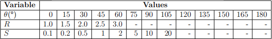
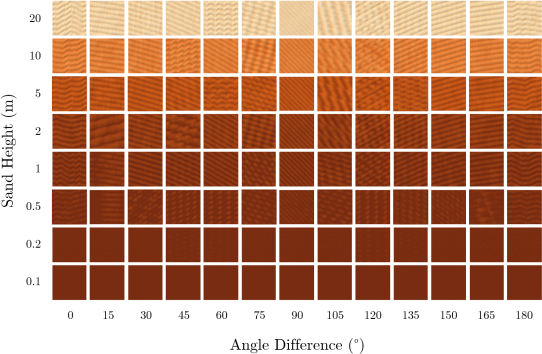
Figure 3.1: Heightmaps for wind ratio, R = 1

3.1.2 Results

Final heightmaps from these simulations are presented below in Figure B.1 for R = 1, and additionally in Appendix A.1 for R = 1.5, 2, 2.5, 3. Note that in these figures the angle difference is clockwise from the dominant wind direction (southbound). The heightmaps are shown using Mathematica’s ReliefPlot function, which uses a combination of the heightmap and a generated hillshade to produce the elevation plots. The color scale is kept the same for each figure.

As can be seen, at low sand supplies, S ≤ 0.2, there is very limited sand dune development as the sand slabs are constantly moved and are not able to settle into a pattern. In Figure B.1, a transition from longitudinal dunes to transverse dunes can clearly be seen when θ > 90, which is as expected as the opposing winds cancel out and push sand into ridges.

However, there are some features which are not as easily explained by sand dune mythologies, such as horizontal and vertical features in A.3, and poorly developed dunes for θ = 0, 180 for R = 1.5, 2.5, 3. Specifics reasons as to why these features are observed are not well understood at this stage, but may likely due to the discrete simulation bounds and grid of the model and do not reflect real or intended behaviours.

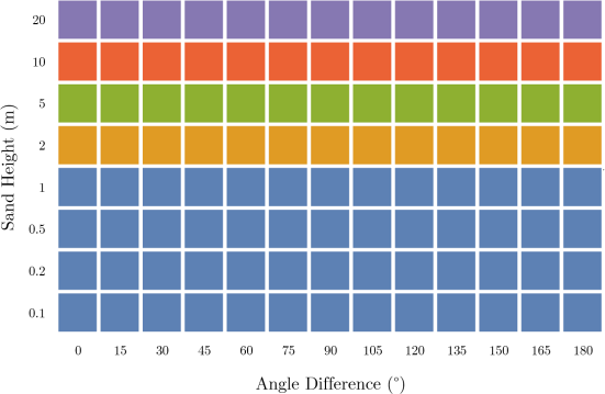
Figure 3.2: Heightmaps for wind ratio, Same for all R

3.2 Classification

As an aim of this project, different wind regimes were intended to be classified into different regions based on the type of sand dune attractor into which the resulting simulation settles. In order to generate reasonable classifications without introducing bias on the side of the author, an unsupervised machine learning approach was suggested as a way of automating the process and to investigate this as a reasonable way of classifying observed dune formations. This was done using Mathematica’s Clustering Analysis tools, specifically ClusteringComponents[].

3.2.1 Clustering based on Heightmap Data

As a first pass, the heightmap data was used to cluster the results with a maximum of 5 groups. This result was not very interesting as it produced an output which was strongly correlated with the mean height of the simulation, refer to figure 3.2.

3.2.2 Clustering based on Interpreted Ridges

The Mathematica symbol RidgeFilter[] is used to estimate the presence of ridges in images. This filter was applied to all the height-maps to determine the dominant Ridge lines within the simulations, ignoring the absolute height. The results of

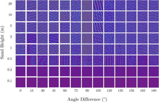
Figure 3.3: Ridges for wind ratio, R = 1

applying this filter are shown in Figure 3.3 for R = 1 and in Appendix A.2 for other ratios. Observing these results, we see that simulations with similar features but different heights have generally similar ridges, indicating that this may be a good fit to use for clustering analysis.

The results of the clustering analysis based on the ridge images is shown in 3.4, and in Appendix A.3 for the other ratios. From this analysis, we can interpret a few regimes that the model has clustered. These can be interpreted as:

• Blue - Poorly developed / no dunes

• Yellow - Barchans or typically linear dunes with lateral separations between dunes

• Green - Longitudinal and Linear Dunes

• Orange - Typically longitudinal dunes with some transverse connections between ridges

• Purple - Similar to Orange, different dominant dune angle.

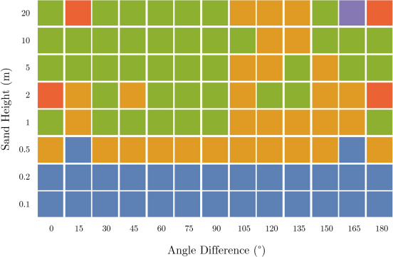
Figure 3.4: Clustered Ridges for wind ratio, R = 1

3.3 Wind Data

The World Meteorological Organization is an agency of the UN which standard-ises and enables the distribution of weather information. Historical wind meas-urements are captured on a regular basis (typically hourly) from these weather stations. Mathematica allows for the extraction of historical data from these sta-tions using the WindSpeedData[] and WindDirectionData[] functions. Using these functions, wind vector data for a year was taken from real weather stations which were nearby sandy deserts. This wind vector data was applied to the sand dune model in order to replicate real life wind data. Mathematica code for this simulation is provided in Appendix D. The wind speed from this model is used as the wind strength factor in the model, e.g. 15 km/h wind = 15 patches transported for each sand slab transported.

3.3.1 Locations

Strzelecki Desert

The Strzelecki Desert is in the far north region of South Australia. This region has pronounced linear dunes as shown in 3.5. There is a nearby weather station as part of the Moomba Airport, which was used for the wind analysis. As can be seen in the wind vector bivariate probability distribution plot in 3.6, the observed wind is typically bimodal, with dominant wind at 130◦and 180◦ . Note that in still conditions, the wind is logged as (360◦ , 0 km/h), leading to the peak in the bottom right.

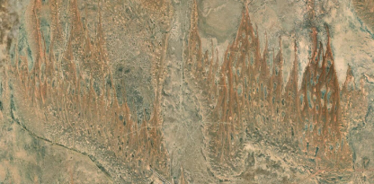
Figure 3.5: Satellite imagery near Moomba Airport depicting linear dunes

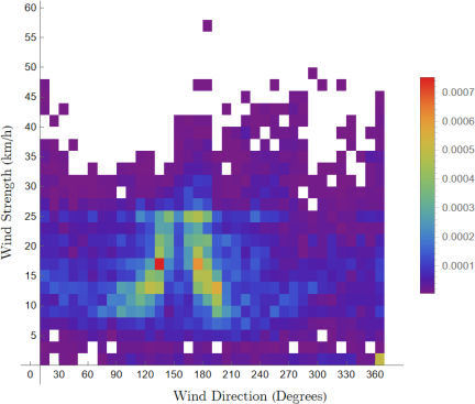
Figure 3.6: Bivariate probability density function for Wind Speed and Direction, Moomba Airport

Taklamakan Desert

The Taklamakan Desert is in northwest China, and is an actively shifting desert, with dunes as can be seen in Figure 3.7. The wind distribution is shown in 3.8.

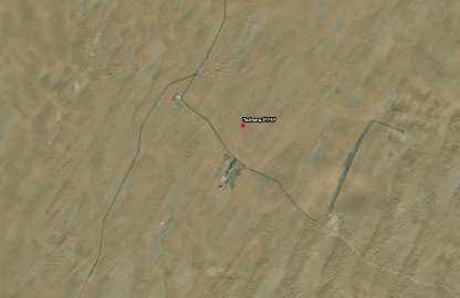
Figure 3.7: Satellite imagery near Tazhong Weather station, Taklamakan Desert, depicting longitudinal dunes

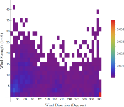
Figure 3.8: Bivariate probability density function for wind speed and direction, Tazhong Weather Station

3.3.2 Simulation Results and discussion

Unfortunately, the results from the wind data did not cleanly replicate the features found in real life deserts. It appears when using a wind regime which is highly variable and sand is allowed to travel in any direction, there is a positive feedback loop which results in the formation of a single dominant mound of sand. This affect may be as a result of the implementation of the "wind shadow", which is based on simple assumptions that do not take into the turbulent, inertial behaviour of wind and behaves the same in any changing direction, for any height of dune. Additionally, it may be due to assumptions in the sand transportation, as there is no minimum speed that is required to pickup a sand slab and deposit it, and other research conflicts with this assumption (Lancaster, 1994). There is also a fundamental lack of definition in the spatio-temporal scale in the Netlogo model, which makes it difficult to justify timescales and sand flux rates to real life data.

Regardless, results from the simulations are shown in 3.9, and 3.10, where it can be seen that although there is the single mound attractor, the mounds that do evolve become elongated in the similar principal directions to what is seen in the satellite imagery.

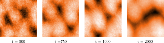
Figure 3.9: Heightmap of Netlogo simulation on Moomba wind data, different simulation ticks t

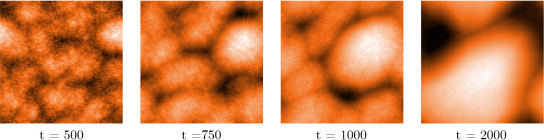
Figure 3.10: Heightmap of Netlogo simulation on Tazhong wind data, different simulation ticks t

3.4 Obstacle Model

The model with the obstacle extension was applied against two situations to judge its effectiveness in replicating assumed behaviour. The implementation of the rigid obstacles is shown to be generally well consistent with assumed behaviours for wind blown sand, as it piles up on the windward face of the obstacles, and generates tails around the sides of the obstacles in the wake of the wind.

3.4.1 Perforated Wall

In the perforated wall model, wind is blown against a tall wall with two perfora-tions. Initially, it can be seen from 3.11 a) that the sand is blocked from progressing past the wall except for the perforated regions, where the sand mounds up around the leeward side of the perforations. In 3.11 b), the sand has built up enough around the windward side of the obstacle to become taller than the wall and be-come deposited on the windward side. In 3.11 c), most of the sand is now on the leeward side of the barriers, and is restricted from moving as it is in the shadow region of the wall.

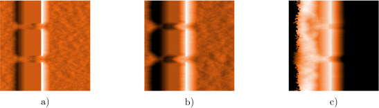
Figure 3.11: Evolution of perforated wall model

3.4.2 Shaped Barriers

In the shaped barriers model, three shapes of barriers (concave, convex and flat) are compared against each other for effectiveness against sand flux coming from a diagonal. As can be seen in 3.12, the concave barrier is able to capture and funnel more of the sand into the apex of the barrier, leading to an early toppling of the sand on the other side of the barrier. The flat barrier is overcome afterwards, and the concave barrier does not result in any over toppling until much later in the simulation, as the wedge shape allows the sand to be distributed away from the apex of the barrier.

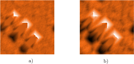
Figure 3.12: Evolution of shaped barriers model

Critical Assessment

4.1 Benefits of the model

The simple model we have implemented in NetLogo has been found to produce the simplest forms of dunes, specifically barchan and linear, which only depend on sand supply and wind strength. We are able to see transitions between resultant dunes based on parameter changes, and used image processing algorithms and experimented using unsupervised learning to classify different dune formations. This model benefits from being a simple model, and can be quickly modified and adapted, and runs generally in real time.

This is different to other contemporary models such as ReSCAL (Rozier and Narteau, 2014), which uses a 3D cubic lattice cellular automaton, and is used in other research (Gao, Narteau et al., 2015; Gao, Gadal et al., 2018; Lü, Dong and Rozier, 2018), to generate more rigorous models as it contains a coupled fluid modelling system.

4.2 The limitations of the model

4.2.1 Validating the model

Our proposed method of validating the model was to use the Mathematica wrapper to run simulations using realistic wind conditions from regions where sand dunes of a specific type are known to form. However, knowing the prevailing wind conditions is only one part of an accurate model for a specific location, the sand availability, amount of vegetation and probability of the growth of the vegetation are also crucial for an accurate model. These additional variables aren’t as easily determined or found as the prevailing wind conditions meaning it would be difficult to fully validate the model for a specific location.

An alternate method of validating our model would be to create phase dia-grams equivalent to those published in articles using other modelling techniques or languages that have themselves been validated. In our proposal we identified a number of publications that contained either models or real-world phase diagrams that we could use to help validate our model. Some of this validation work has been attempted but a rigorous validation incorporating more modelling loops and extensions could not be completed due to the time constraints of this project.

4.2.2 The size of the world

Most of our runs were performed with a world size of 100x100 patches, at this size it would take between approximately 1 second per tick to run at the fastest setting on a reasonably fast computer. Increasing the world size to 500x500 patches increased that to 2-3 seconds per tick. Although it did depend on the settings, it would generally take 1000-1500 ticks for recognisable dunes to form which is approximately 1 hour at the larger world size. While an hour per run would be ok for validation or results formation it wasn’t useful for testing and parameter sweeping hence the choice to go with the smaller world size that was a good compromise between run time and world size. This smaller world size may have introduced boundary effects as deposition of sand slabs at higher speeds would be frequently wrapping over the world boundary.

4.2.3 Implementation of physical distances

Though our model purports to use physical distances such as meters of sand, and meters per second for wind speed, it is simply using a linear relationship between the parameters. This is substantially due to the lack of understanding what a ‘tick’ is equivalent to in the real-world. Theoretically if the flux of sand passing a spot was known for an area this could be used to calibrate a tick to an actual length of time. This would also help to ground the growth rate of vegetation.

4.2.4 Every patch is acted on every tick

The model assumes every patch that isn’t shadowed has a slab of sand eroded and moved forward each tick. It isn’t clear if this is consistent with reality or not, but it is the default in all previous models that we found.

4.2.5 Effect of increasing wind speed

The model assumes that increasing wind speed has a simple linear effect on how far the sand is transported before deposition. It’s likely that an increase in wind speed has a non-linear impact on sand erosion, travel distance, and deposition probability.

4.2.6 Sand transport

Currently the model assumes the sand is transported in a straight line from source to destination regardless of what is in the path. This is likely only true for a flat plain, as soon as dunes form the wind would flow around and through them changing this straight-line assumption and likely increasing deposition at the base or sides of a dune where the wind changes direction (particularly in low wind conditions). A more accurate model would couple the wind deposition vector with the elevation.

4.2.7 Vegetation growth

We have implemented a very simple vegetation component to the model where the whole patch becomes vegetated and ‘fixed’ if vegetation grows on it. This is based on a fixed percentage for a patch without sand and 0.01 of that percentage for patches with sand. This is highly unlikely to be equivalent to reality due to the overly simple nature of the implementation.

4.2.8 Sand supply

We have assumed that sand supply can be modelled using mean-initial-depth; a lower mean depth of sand leads to a lower supply. This decision is largely justified in that we have been able to largely replicate the phase diagrams from literature showing expected dune type for a range of wind conditions and sand supply. However, it is also a simplistic implementation that is strongly dependant on the slab height used in the model and the wrapping world boundaries. An alternate way of modelling sand supply would have been to not wrap the world boundaries and each tick introduce a percentage of sand from the specified wind direction. This method would, in some respects, be closer to what happens in reality however it also has its own drawbacks.

4.2.9 Obstacle model

The obstacle model was implemented on a modified version of the full model with vegetation removed and less variables available for modification. It was done this way to simplify the model and make it easier to implement the obstacle detection.

Obstacle detection is performed by moving the slabs of sand in 0.5 patch in-crements until the full move distance is reached checking at each step whether an obstacle had been encountered. This method of moving the slabs of sand is inefficient and the time required per tick increases with the size of the wind-speed, along with the total number of patches. One potential way of avoiding this in-crease would be to model the movement of a slab of sand using a turtle, this would give access to additional functions that aren’t usable with patches.