Mathematica

Hello, dear friend, you can consult us at any time if you have any questions, add WeChat: daixieit

PART A

Show all working

1. (a) If (A − C) log10 = 7.32 Q + 1, find X in terms of A, C, P and Q.

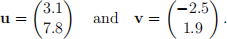
(b) Let

Find u.v and hence find cos θ where θ is the angle between u and v. Find θ, expressed in degrees.

(c) Write e2i in the form a + ib.

(d) Let

Find (A − BT)C.

(e) Consider

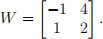
Find both the eigenvalues of W and the eigenvector corresponding to each eigen-value.

(f) is a function of the independent variable, k. Find .

PART B

Show all working and provide Mathematica code when you use Mathematica.

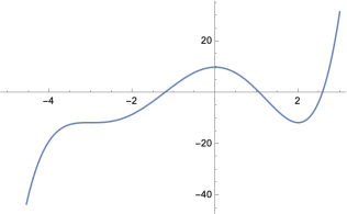
2. (a) The sketch below shows the graphs of x = f(t). Sketch the graph of the first and second derivatives of f(t) in separate diagrams. Mark on your sketches any noteworthy features and explain how these are linked to the graph of x = f(t).

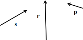
(b) Consider the geometric vectors s, r and p shown below. Find the geometric vector s − r + p.

(c) Use Mathematica to find N(M +K)3 where K, M and N are given below. Express the elements of the matrix that you find in scientific notation, correct to three significant figures. (When Mathematica has found the solution, it is perfectly acceptable to write down the final answer with pen and paper so that it is in the correct format.)

(d) You have been given a file Assignment2data.nb on the Assignment 2 page. This file contains data from an experiment that measures a dependent variable S in grams as a function of time t in seconds. According to theory S and t are linked by the equation . Find values of S0 and that fit this data. On the same set of axes, plot the data and the curve , using the values of and S0 that you have found.

3. Orca population dynamics on Canada’s west coast. This question relates to the scientific paper ”Pod-specific Demography of Killer Whales (Orcinus orca), by Brault and Caswell, published in 1993 in Ecology. You can download this from the Assignment 2 page on Canvas.

Orcas are also known as killer whales, although this term has become old-fashioned now. They live in large family groups called pods.

The paper by Brault and Caswell uses existing data to construct a stage-based Leslie matrix model for orcas that live in the American Pacific Northwest, o↵ the coast of Canada and Washington state. Brault and Caswell call this a projection model as it emphasises what will happen if nothing changes to the system, rather than predicting what actually will happen.

The time interval (or“tick of the clock”) in this model is one year. In the paper, this is called the projection interval.

In a stage-based model, individuals can stay in one or more of the classes for more than one time interval. For example, in this model, individuals can remain in the juvenile class (class 2) for about 14 years and in the mature class (class 3) for about 20 years.

The model here only considers female orcas. This is a common approach in many popu-lation models as population dynamics tend to be driven by the numbers and behaviours of females, rather than males.

It will help you if you read at least some of the paper, but you do not need to read it all. As you might expect, it includes the use of techniques that we do not study in this unit, including statistical techniques. However, the Introduction and the Discussion are useful as these sections put the research in context and help you understand some of the terminology of the rest of the paper.

(a) The life-cycle graph for the female orca population is given at the top of the second column on page 1446.

(i) What do the di↵erent classes represent?

(ii) Explain why there are loops on this graph that leave each class and then return to the same class.

(iii) What does the model assume about what each class does? Explain these assumptions, either in words or by labelling the arrows on the graph.

(b) The Leslie matrix (projection matrix) that corresponds to the life cycle graph is shown just below the graph n page 1446.

(i) Explain why the first element in the first row is zero.

(ii) Numerical values for non-zero elements of the Leslie matrix are given in the matrix A at the top of page 1447. Enter this matrix into Mathematica and find the eigenvalues and eigenvectors. What is the largest real (that is, not complex) eigenvalue of the Leslie matrix? Write this down and its corresponding eigenvector.

(iii) We know that this largest real eigenvalue (known as the dominant eigen-value) gives the rate of growth from one year to another. From the value for the dominant eigenvalue that you have found, what is the yearly relative rate of growth for this orca population, given as a percentage?

(iv) Find the sum of the elements of the eigenvector that corresponds to the largest positive eigenvalue that Mathematica has found. We will call this sum D so that we can refer to it easily. Divide each element of the vector that Mathematica has found by D. When you do this, you should get the vector w given in equation (5) on page 1448.

(Note that this paper also refers to other information that can be obtained from the Leslie matrix, such as elasticity and reproductive value. These are very useful, but are not covered in MATH1050.)

(c) Let us consider a population that, at t = 0 has 10 female yearlings, 62 immature female orcas, 68 female orcas of reproductive age and 39 post-reproductive females. Construct a vector that represents a population with this structure. Using the Leslie matrix A, find the population in each class at each time from t = 0 to t = 8. Use ListPlot to plot these populations for these times. (You may want to think about use of colour in your graph and/or joining the dots for each class to make sure that you are communicating well with your reader. You can find out how to do this from Mathematica documentation on the web or via AI.)

(d) (i) In the paragraph directly under the heading “Matrix Analyses” on page 1447, the authors make this statement: “The asymptotic rate of population growth is given by the dominant eigenvalue λ of the matrix A; the corre-sponding continuous time rate r = ln λ.” Using this information, write down a model for the continuous growth of the total population where the initial population is as described in the previous part.

(ii) Plot the predictions for total population size from the continuous model and from the matrix model on the same plot. (Note that the continuous model is plotted as a curve and the matrix model will be plotted as a series of points at discrete time intervals.) Do they agree? Why or why not?