关键词 > IEOR242
IEOR 242: Applications in Data Analysis, Spring 2021 Practice Midterm Exam 2
发布时间:2024-06-29
Hello, dear friend, you can consult us at any time if you have any questions, add WeChat: daixieit
IEOR 242: Applications in Data Analysis, Spring 2021
Practice Midterm Exam 2
March 2021
1 True/False and Multiple Choice Questions – 48 Points
Instructions: Please circle exactly one response for each of the following 16 questions. Each question is worth 3 points. There will be no partial credit for these questions.
1. In logistic regression, it is assumed that the dependent variable Y corresponds to a probability value in the interval [0, 1].
A. True
B. False
2. Consider a previously trained logistic regression model for predicting whether images correspond to cats or dogs. If p denotes the model’s prediction of the probability that a new image is a dog, then it must be the case that 0 < p < 1.
A. True
B. False
3. The probability model underlying logistic regression includes an assumption that the feature vector X comes from a multivariate normal distribution.
A. True
B. False
4. The probability model underlying linear discriminant analysis (LDA) includes an assumption that, con- ditional on observing the value of the dependent variable (i.e., Y = k for some k ∈ {1, 2, . . . , K}), the feature vector X comes from a multivariate normal distribution.
A. True
B. False
5. If we use k-fold cross validation on a training set to select a final model, then there is no need to evaluate the performance of this model on a test set since it is impossible for this model to overfit the training set.
A. True
B. False
6. One of the main reasons that boosting is efective is because, at every iteration, the algorithm finds a new decision tree that is very large (i.e., its depth is very big).
A. True
B. False
7. Consider a training set with n = 1000 data points. Then, using 10-fold cross to select the cp parameter in CART is roughly 100 times cheaper in terms of total computation time than using leave-one-out cross validation.
A. True
B. False
8. Due to the random initialization, it is possible for the K-means algorithm to return diferent cluster assignments on the same dataset.
A. True
B. False
9. It is not possible to train an LDA (linear discriminant analysis) model on a dataset that includes one or more categorical features.
A. True
B. False
10. Consider a time series Xt for t = 1, 2, . . . T. Then the correct model equation for an auto-regressive model is Xt = β0 + β1t + Xt — 1 + Et where β0 and β1 are unknown coe伍cients that must be trained from the data and Et is the error term.
A. True
B. False
11. The Zipf distribution of word frequencies has a light tail that decays exponentially fast. In other words,
uncommon words make up a very small percentage of all of the text in a typical document corpus.
A. True
B. False
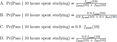
12. Consider a binary classification problem for predicting whether or not a student will pass a midterm exam based on how many hours the student has spent studying. Suppose that 90% of students will pass the exam, and 10% will fail. Given that a student will pass the exam, the number of hours spent studying is a continuous random variable with density function fpass (x). Likewise, given that a student will fail the exam, the number of hours spent studying is a continuous random variable with density function ffail (x). Which of the following is a correct expression for Pr(Pass j 10 hours spent studying), the probability that the student passes given 10 hours spent studying?
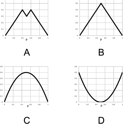
13. Consider the CART algorithm for binary classification. A desirable property of an impurity function for the CART algorithm is that a split never increases the total impurity cost of the tree (i.e., using the notation from class we have △ ≥ 0). Figure 1 below depicts four potential impurity functions that might be used in CART, each as a function of the proportion p of observations with Y = 0 in the current bucket. Which of these impurity functions have the desirable property mentioned above?
A. All four
B. Only A, B, and C
C. Only B and C
D. Only C
Figure 1
14. In a binary classification problem, an efective method for building a model and generating a confidence interval for its T P R (true positive rate) is to first split the entire dataset into a training set and a test set and then:
A. Train the model on the training set, then use the bootstrap on the entire dataset
B. Train the model on the training set, then use the bootstrap on the training set
C. Train the model on the training set, then use the bootstrap on the test set
D. Train the model on the entire dataset, then use the bootstrap on the test set
15. Consider the following ROC curves for two diferent models – the “dashed model” whose ROC curve is the dashed curve, and the “solid model” whose ROC curve is the solid curve. The baseline is also drawn for comparison. Which statement below is a correct interpretation of these ROC curves:
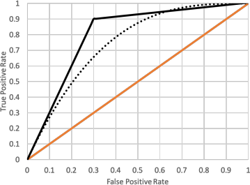
A. Since the AUC of the solid model is greater than the AUC of the dashed model, the solid model is always preferable over the dashed model
B. If we desire a model with FPR between 0.8 and 0.9, then the solid model is strictly preferable over the dashed model
C. If we desire a model with TRP between 0.8 and 0.9, then the solid model is strictly preferable over the dashed model
D. None of the above
16. A linear regression model was trained on a training set of size 145, and estimates of OSR2 (out-of- sample R2 ) and MAE (mean absolute error) were computed on a test set of size 63. The test set OSR2 is 0.732 and the test set MAE is 38.5. The bootstrap was then used in order to estimate the bias of the estimates of OSR2 and MAE. First, B = 10, 000 bootstrap datasets were used, then a second analysis with B = 1, 000, 000 bootstrap datasets was done. The results are summarized in the table below.
|
|
Bias of OSR2 (Bootstrap Estimate) |
Bias of MAE (Bootstrap Estimate) |
|
B = 10, 000 |
0.0300 |
0.223 |
|
B = 1, 000, 000 |
0.0297 |
0.00927 |
A correct interpretation of these results is:
A. Both the OSR2 estimate based on the test data and the MAE estimate based on the test data are most likely unbiased.
B. Both the OSR2 estimate based on the test data and the MAE estimate based on the test data are most likely biased.
C. The MAE estimate based on the test data is most likely unbiased, but more bootstrap samples (B >> 1, 000, 000) are needed to determine if OSR2 is biased or not.
D. The MAE estimate based on the test data is most likely unbiased, whereas the OSR2 estimate based on the test data is most likely biased.
2 Short Answer Questions – 52 Points
Instructions: Please provide justification and/or show your work for all questions, but please try to keep your responses brief. Your grade will depend on the clarity of your answers, the reasoning you have used, as well as the correctness of your answers.
1. (20 points) This problem concerns a computer hardware dataset from the 1980s with n = 208 obser- vations, each corresponding to a diferent CPU (central processing unit) model. For each CPU model, the dataset includes a variable called PRP, which is a measure of the relative performance of that CPU model as compared to a particular baseline model as published by a magazine. We are interested in predicting the PRP value of a CPU model based on its basic attributes. Table 1 below describes these attributes in more detail.
Table 1: Description of the dataset.
Variable Description
|
MYCT |
Machine cycle time in nanoseconds |
|
MMIN |
Minimum main memory in kilobytes |
|
MMAX |
Maximum main memory in kilobytes |
|
CACH |
Cache memory in kilobytes |
|
CHMIN |
Minimum channels in units |
|
CHMAX |
Maximum channels in units |
|
PRP |
Published relative performance |
Summary statistics for the full dataset are provided below:
The dataset was split into a training set with 145 observations and a test set with 63 observations, and a linear regression model was built, using the training data, to predict PRP based on the five independent variables. The output from R is given below.
Please answer the following questions.
(a) (4 points) A CPU manufacturer is considering a new model with machine cycle time of 75 nanosec- onds, minimum main memory of 2,500 kilobytes, maximum main memory of 10,000 kilobytes, cache memory of 30 kilobytes, a minimum of 4 channels and a maximum of 8 channels. Use the R output on the previous pages to make a prediction for the published relative performance of the proposed CPU model.
(b) (4 points) Is there a high degree of multicollinearity present in the training set? On what have you based your answer?
(c) (4 points) Based on the R output on the previous pages, is there enough evidence to conclude that the true coe伍cient corresponding to CHMAX is not equal to 0? On what have you based your answer?
(d) (4 points) Consider adding a new independent variable to the model called CHAVG, which is defined as CHAVG = (CHMIN + CHMAX)/2. Is it possible for this new variable to improve the linear regression model for predicting PRP? Explain your answer.
(e) (4 points) Consider adding a new independent variable to the model called CACHSQUARED, which is defined as CACHSQUARED = (CACH)2 . Is it possible for this new variable to improve the linear regression model for predicting PRP? Explain your answer.
2. (10 points) Please answer the following two questions concerning Bagging and Random Forests.
(a) (5 points) Andrew has ambitiously tried to write his own code for Bagging (Bootstrap Aggregation)
of CART models. Unfortunately, he has a bug in his code when generating the bootstrap datasets because he accidentally implemented sampling without replacement (instead of sampling with re- placement). You may assume that there are no other bugs in the Bagging code. Andrew is now preparing to run some experiments on several diferent datasets (both regression and classification problems) in order to compare the test set performance of his Bagging implementation with that of the basic CART method with cp = 0 and all other parameters set to their default values. You may also assume that these other parameters for CART are set to the same default values within the Bagging code. What do you expect the results of Andrew’s experiments to be? In other words, how do you expect the test set performance of Andrew’s Bagging implementation to compare to that of CART with cp = 0? Briefly explain your response.
(b) (5 points) Meng has now decided to write her own code for Random Forests, using Andrew’s code with the same bug (sampling without replacement instead of sampling with replacement) as a starting point. You may assume that there are no other bugs in her Random Forests code and that mtry (a.k.a. m) is set to something less than the number of features p. Meng is now preparing to run some tests on several diferent datasets (both regression and classification problems) in order to compare the test set performance of her Random Forests implementation with that of the basic CART method with cp = 0. What do you expect the results of Meng’s experiments to be? In other words, how do you expect the test set performance of Meng’s Random Forests implementation to compare to that of CART with cp = 0? Briefly explain your response.
3. (22 points) In this problem, we will revisit the Lending Club loans .csv dataset from Lecture 3. Recall that we would like to build a model to predict the variable not.fully.paid (which is equal to 1 if the borrower defaults on the loan) based on the given six independent variables, which are summarized in Table 2 below.
Table 2: Description of the dataset.
Variable Description
|
installment |
Monthly loan installment in dollars |
|
log .annual .inc |
Log(annual income) |
|
fico |
FICO score |
|
revol .bal |
Revolving balance in thousands of dollars |
|
inq .last .6mths |
Number of inquiries in the past six months |
|
pub .rec |
Number of deleterious public records |
|
not.fully.paid |
Equal to 1 if the borrower defaults on the loan |
Recall that a positive observation corresponds to someone who defaults, i.e., not.fully.paid = 1. We will consider the same scenario as in class, whereby we lose $4,000 every time a borrower defaults on a loan, and we gain a profit of $1,000 every time a borrower does not default. This scenario is summarized by the decision tree shown in Figure 2 below.
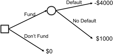
Figure 2: Simple Lending Decision Tree
In this problem, we will consider applying CART and Bagging on this dataset.
Please answer the following questions.
(a) (6 points) Determine specific numerical values of LFP and LF N such that training a CART model in order to minimize
LF N (# of False Negatives) + LFP (# of False Positives)
is the same as training a CART model in order to maximize total profit, and explain why the two are equivalent.
A CART model was trained using the values of LFP and LF N determined in part (a) above. The tree corresponding to this model is displayed in Figure 3. Recall that a prediction of not.fully.paid = 1 corresponds to a “bad risk,” and a prediction of not.fully.paid = 0 corresponds to a “good risk.”
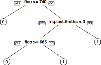
Figure 3: CART Tree
Use the CART tree above to answer the following two questions.
(b) (4 points) Consider a new potential borrower with a FICO score of 650, and suppose that no other information is known about this borrower. Does the CART model above classify this borrower as a good risk or a bad risk? Explain your answer. If you do not have enough information about the borrower to answer this question precisely, then explain what additional information is needed and how this additional information afects the classification of the model.
(c) (4 points) Consider a new potential borrower with 4 inquiries in the past six months, and suppose that no other information is known about this borrower. Does the CART model above classify this borrower as a good risk or a bad risk? Explain your answer. If you do not have enough information about the borrower to answer this question precisely, then explain what additional information is needed and how this additional information afects the classification of the model.
(d) (4 points) Let us consider applying Bagging (Bootstrap Aggregation) of CART trees for this prob- lem. Suppose that we construct B diferent bootstrap training sets, and for each bootstrap training set we train a CART model using the standard choice of LF N = LFP = 1. In this case, the propor- tion values in each bucket can be used to define probability estimates. Given a new feature vector x corresponding to a new potential borrower, let f^b (x) denote the prediction of the probability that this borrower will default by the bth CART model. Explain precisely how you would use the predicted probability values f^1(x), f^2(x), . . . ,f^B(x) to classify the new borrower as either a good risk or a bad risk.
(e) (4 points) Repeat part (d) instead under the assumption that each CART model is trained using the values of LFP and LF N determined in part (a) (instead of LF N = LFP = 1). For this question, you should also instead assume that f^b(x) is the classification of the borrower as either a good risk or a bad risk. That is, f^b(x) takes the value of either 0 or 1.
