Elec4622 Laboratory Project 1, T2 2024

Hello, dear friend, you can consult us at any time if you have any questions, add WeChat: daixieit

Elec4622 Laboratory Project 1, T2 2024

June 12, 2024

1 Introduction

This is the first of three mini-projects to be demonstrated and assessed within the regular scheduled laboratory sessions. This project is officially due in your Week 5 laboratory session, but for this first project only, there will be an opportunity to get assessed or re-assessed in Week 6. Note that there is no possibility to further extend submission of your work beyond Week 6, which is already effectively an extended submission date. Moreover, in order to qualify for assessment or re-assessment in Week 6, you must have uploaded all initial work on the project to a Moodle-based submission portal by the end of your laboratory session in Week 5.

The project is worth a nominal 10 marks, out of the 30 marks available for the laboratory component of Elec4622. However, there are optional elements which can attract a lot of bonus marks! You will probably not do all the optional elements, although you are welcome to try. In any event, some bonus marks can really help you a lot down the track, so you are recommended to attempt at least some of the options.

In this project you will design and implement Gaussian and related filters to extract edge-related information from an input image at various scales. Gaussian filters have some very nice propertie that have been studied in lectures and at least one tutorial question so far, so you should revise that material from your lecture notes first. You may also find it useful (though not essential) to read the "Image Analysis" chapter of your typeset lecture notes for the course.

To do the project, you should read the following notes very carefully, drawing lots of diagrams on your own to help ensure that you understand what is going on. You will find that details are very important. This is critical for your development as an engineer- engineers know how to go from a general big picture down to the details. Running high level functions, such as one often does in Matlab, does not lead to a deep understanding, since it conceals so many of the details from view. In this project, you are forced to come to grips with the details and that is exactly what employers want from graduates that they employ.

Get ready to put a lot of work into this project, but also to learn a huge amount from it!

2 Gradients, Derivatives and Differences of Gaussians

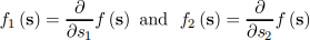
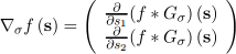
An important operation in image processing is differentiation. Consider a continuous image f(s), with horizontal and vertical derivatives

Then the gradient vector for f(s) is written

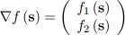
and takes values at each spatial location.

The magnitude of the gradient vector

is the maximum rate of change of the image intensity f(s) in any direction, while the orientation of Vf (s) is the direction associated with this maximum rate of change. To see this, let & denote a small change in spatial position s; then the rate of change of intensity in the direction of o is

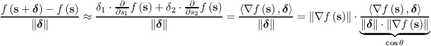
The last term on the right hand side of the above equation necessarily lies in the range -1 to 1, by the Cauchy-Schwartz inequality, and is in fact just the cosine of the angl O between Vf (s) and &.  So when the direction of movement is the same as the gradient vector Vf (s), we observe the largest rate of change in intensity, which is |▽f (s)|. Differentiation is an LSI operator, so it is equivalent to multiplicatoin in the Fourier domain.  In particular, it is easy to show that

Therefore, true differentiation of an underlving bandlimited continuous image can be implemented preciselylby applying discrete LSI filters hi [n] and h2 [n] to the discrete image z [n] = f(s)s=n, where

This allows us to compute the true gradient vector of the underlying continuous image at each discretelocation n, simply by convolving by hi and h2.

Not suprisingly, the PSFs h and h have infinite support in space, so must be approximated. Onesimple approach is just to take the inverse DSFT of hi and h2 and apply a raised-cosine (Hanning) windowto obtain finite support approximations to the derivative operators. In fact, the ideal filters obtained bytaking the inverse DSFT of hi and h2 are given by

Very simple approximations to these differentiation filters can be obtained by using

Make sure you understand what these trivial approximations, each with only 2 non-zero coefficients, are actually doing and how to implement them. In particular, use a pen and paper to sketch out what happens if you perform convolution with these filters, using the output perspective to show that these are just calculating simple "finite differences" on the input image. It is also instructive to work out the Fourierl transform of these 1D horizontal and vertical filtering operations; in particular,

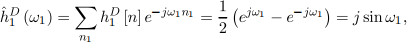
which is approximately equal to jwi for small wi.Notice that the ideal differentiation filters hi (w) = jwi and hi (w) = jw2 are strongly high-pass, with magnitude responses that increase linearly with wi and w2, respectively. For this reason, it is common to combine differentiation with low-pass filtering operation, where the amount of low-pass filtering determines the "scale" at which gradients are obtained. In particular, Gaussian low-pass filters are strongly desirable, due to their rotational symmetry and other properties. In this way, we can determine a scale-dependent gradient

where Go is a circularly symmetric Gaussian low-pass filter with standard deviation o, which is alsounderstood as the "scale parameter."In lectures you learned how to perform Gaussian filtering on discrete images while ensuring that theresult is equivalent to Gaussian convolution on the underlying continuous image. You will be doing thisin this project and combining Gaussian filtering with derivative approximations, in order to discover anddisplay gradient orientation within images.

3 Second derivative operators

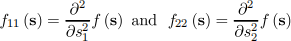
Since you now know how to differentiate an image, the approach can readily be extended to a second level of differentiation. Again, write f(s) for the spatially continuous image, with horizontal and vertical second derivatives

Then the Laplacian operator can be written as

In the Fourier domain, we have

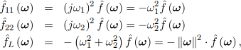
which reveals the fact that the Lapacian operator is a circularly symmetric filter in the continuous domain.One particularly important property of the Laplacian filtered image is that the precise locations ofimage edges correspond to zero-crossings of fz (s) - i.e., the zero-valued contours of the function fz (s).

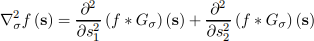
As with differention (in fact much more so), second derivative operators are strongly high-pass, sol it is again common to combine the Laplacian operator with a Gaussian low-pass filter. This leads to al scale-dependent Laplacian operator, which we can express as

4 Boundary and image extension

As you already know, image boundaries cannot simply be ignored. In this project, you will use filters with various regions of support, so from a practical perspective you must ensure that the output image dimensions do not depend on how large the filter support is. Unless otherwise stated, you should use the symmetric boundary extension method.

5 How to go about the tasks

These notes assume that you will demonstrate your work using the laboratory PCs, based on the Windowsl operating system with Microsoft Visual Studio. You may use your own personal computer to develop code and also to demonstrate your work, but it will be more time efficient for laboratory demonstrators to assess your project on the laboratory PCs, which may result in you getting more opportunities to correct errors in your solution and be re-assessed for particular tasks. In general, if you make thingsl easier for the lab demonstrators, they will be able to make things easier for you.

For demonstration purposes, you should create a separate project for each task, within a single workspace. You can do this by using the "File→ New→ Project" option in Visual C++, replacing the "Create new solution” option with "Add to solution”.

Be sure to arrange for all your executable programs to be placed in a single location (e.g.,c:(elec4642(bin), which is referenced from the path environment variable. Also, please place all the images you are working with into a single directory (e.g., c:\elec4642)data). That way, it will be much easier to demonstrate your work in a time effective manner-it will also save you personally a lot of time. In any event, you might not be marked for your work unless it is organized in this way.

You are required to produce hand-drawn sketches illustrating key features of your design for each task. This is not really any additional work, since it would normally be part of the process of coming up with a design and getting it working. As explained already in laboratories, being able to draw what a diagraml of what your program is doing is an essential first step to implementing a solution and a key element in the debugging process. Do not discard these sketches and diagrams, since lab demonstrators will ask to see them when marking your work, and you are also required to upload them to Moodle as part of an electronic submission process for the project.

You should rely primarily on mi viewer for viewing images, rather than the Windows previewer. There are lots of reasons for this, but the obvious ones are that you can launch multiple copies to viewl multiple images at once, and you can zoom in and inspect individual pixel values with ease. Ultimately, it is a great deal faster and less confusing to execute your programs and view your images directly from the DOS prompt, than by using mouse clicks-assuming you can type. Remember that the up and down arrows allow you to scroll through and edit previous commands easily. Remember also that you can use the tab key to expand file names, program names, etc., so you rarely have to type everything in full.

One thing you need to be prepared for is that it may be difficult at first to know whether your program is working correctly. This is a real world dilemma that you need to learn how to address. Just because your program compiles and produces something which looks like an image does not mean it is doing the right thing. So you need to have a good feeling for what the result should look like, based on your understanding of the fundamental concepts, such as shift and rotation invariance.

To debug your program, you may find it useful to process very tiny images with only a few samples, so you can check that the output is as expected; you can use something like "mi_pipe2 -i image.bmp -o tiny.bmp -form bmp crop_n_shuffle -crop o o 16 16" to create a 16x16 image by cropping a much bigger one. You can also read the sample values directly within the "mi_viewer" application by zooming in (z accelerator) and holding the mouse button down. Then you can see exactly what is going on and match up the results with what you expect from the theory.

To verify your work, it may be helpful to collect sequences of command-line statements together into a script that you can run quickly. You can do this with a Windows batch file (i.e., any file with the ".bat" suffix), which can then be executed like any other program from the command-line. This will greatly facilitate the marking for demonstrators, who might insist upon it.