ECON 23950: Economic Policy Analysis Problem Set 6

Hello, dear friend, you can consult us at any time if you have any questions, add WeChat: daixieit

ECON 23950: Economic Policy Analysis

Problem Set 6 - The Last One

1 Lucas model (1972)

In class, we analyzed Lucas’ model (1972) with zero technological change. Here, we are going to follow exactly the same model (same notation) but we will assume that technological progress grows at a constant rate ϕ :

At = (1 + ϕ)At−1 ⇐⇒ At = (1 + ϕ) tA

where A0 = A and the production function now is

Yi,t = AtLi,t

In log-terms,

at = log(At) = log(1 + ϕ) + log At−1 ≈ ϕ + log At−1

or alternatively:

at ≈ ϕt + a

Moreover, population grows at constant rate n :

Nt = (1 + n)Nt−1 ⇐⇒ Nt = (1 + n) t

Therefore, we can write the main equations derived in class (in log-space):

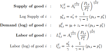
where a 0t = γ−1/γ at .

Note that everything is as in class, but here we do not impose ϕ = n = 0.

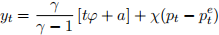
1. Show that the equilibrium level of output of this economy is given by:

2. Define Potential Output (This is when the expected price is equal to the actual price).

3. Define Output gap. You should think of it as a percentage deviation from the poten-tial/natural level of output. Express it in logged variables.

4. Compute the log of Potential Output for this economy, yt*.

(a) In class, we saw that potential output was constant. Is it still true in this case? Why?

(b) Plot the log of potential output over time.

5. Compute the log of potential/natural level of employment, lt*. Is it constant over time?

From now on, assume that population growth is given by n = γ−1/ϕ

6. Show that the (log) employment/population ratio AT THE POTENTIAL LEVEL, log (Nt/L*), is constant over time.

7. Is natural rate of unemployment ut* constant over time? Why? Do not compute it.

8. What is the growth rate of log of potential output per capita?

9. Re-write the aggregate supply in the log space in terms of the output gap and the inflation gap,πt − πte:

10. Define Okun’s law.

11. Using the Okun’s law and the aggregate supply of the economy, derive the Phillips curve in terms of unemployment rate. Plot it.

12. Describe in words the Phillips curve. Does the Phillips curve imply any causal relationship? Explain.

2 Cagan’s Model for Money and Inflation

Suppose that the money demand equation is formulated in the following way:

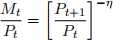
where η > 0 is a parameter.

1. Discuss the interpretation of the money demand equation. Does it make sense? How is it different from a more general money demand equation?

2. What is the interpretation of η? Explain.

3. Take logs on both sides and derive the following expression where pt ≡ ln Pt ; mt ≡ ln Mt :

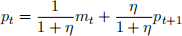
Explain the equation intuitively.

4. Solve the equation forward and express pt as a function of future money supplies. Describe and explain the transversality condition.

5. Suppose that mt+1 − mt = µ for all t = 0, 1, 2, ... (what does this mean?). What is the rate of inflation in this economy?

6. Suppose that the economy had a constant µ = 10% and that one day the central bank announces that from that day onward, µ = 15%. How does the price level (in log) behave over time? Describe the trajectory and explain.

3 Reading Unconventional Monetary Policy

Read Unconventional Monetary Policy in the Great Recession and Beyond and answer the following questions:

1. Describe briefly what the “large scale asset purchases” and “forward guidance” are.

2. How is the “Odyssean” approach different from “Delphic” in term of the transmission mechanism of forward guidance?

3. Explain in your own words how the Fed’s LSAP policy should in theory affect real economic activity.

4. Briefly summarize some empirical evidence on the effectiveness of the unconventional pol-icy.

5. What are some downside risks of the unconventional policy? Describe them briefly.

4 Optimal Monetary Policy with Different Objective Functions

In this question, we use a modified quadratic loss function to think about the so-called discre-tionary and rule-based monetary policy. Assume that the short-run behavior of the economy is captured by the following Phillips curve

u = u* + k(π e − π)

where u is unemployment, u ∗ > 0 is the natural rate of unemployment, π e is the expected inflation, π is the actual inflation, and k > 0 is an exogenous parameter. We assume that the central bank directly controls π.

The central bank faces an inflation-unemployment tradeoff as described by the above Phillips curve. It prefers a low unemployment rate but it also likes stable prices. We capture this tradeoff by specifying the following utility function for the central bank:

V = −[(u − u*)2 + (π − π*)2]

where π ∗ > 0 is the desired rate of inflation.

Let’s assume that the inflation expectations, π e , are fixed for now. The central bank takes the public’s expectations as given.

1. Is there a magic number for π ∗ from the Fed’s perspective? Why is it positive?

2. Interpret intuitively the objective function of the Fed. In particular, why does it depend on the squared deviations instead of squared rates themselves?

3. Set up the central bank’s problem and solve for the optimal inflation rate and unemploy-ment rate, denoted by ˆπ and ˆu, respectively as a function of πe, π*, u*, and k.

4. Suppose that a structural change in the labor market happens (for example, underwater mortgages restrict job seekers’ mobility) such that u ∗ rises. What would happen to ˆu and ˆπ? Explain your results intuitively.

5. Assume that the public has rational expectations and full information, and hence correctly guesses the inflation rate that will ultimately be implemented by the central bank. Solve for the (Nash) equilibrium outcome with its inflation denoted by ¯π and its unemployment ¯u. Interpret the outcome.

6. Can the central bank do better than the Nash Equilibrium outcome? If not, explain why. If so, describe a policy that improves the outcome.

Suppose that the central bank has a more general utility function such that

V = −[(u − u*)2 + θ(π − π*)2]

where θ represents the relative weight that is attached to unemployment deviation, relative to inflation deviation.

7. Do the results in (c)-(f) change? In whay ways?

8. How should we think about inflation targeting in this model? Does it result in the optimal outcome? Explain. (You don’t have to do this question. We will discuss it in class during Week 10.)

5 (Bonus/Optional) Econtalk: Jennifer Burns on Milton Fried-man

Russ Roberts recently had a conversation with Jennifer Burns of Stanford University, who recently published a biography of Friedman. You can find the link here. I believe you’ll find the episode enjoyable, as they delve into some of the contributions of Chicago economics that we discussed in class. Enjoy!