关键词 > MATH2010

MATH2010 Statistical Modelling I SEMESTER 2 EXAMINATION 2020/21

发布时间：2024-06-17

Hello, dear friend, you can consult us at any time if you have any questions, add WeChat: daixieit

MATH2010 Statistical Modelling I

SEMESTER 2 EXAMINATION 2020/21

1. [Total 32 marks] Consider the no-intercept model where

Yi ~ N (βxi , σ 2 ) ,

independently, for i = 1, . . . , n.

(a) Find the least squares estimator,β(^)LS , of β and show that it can be written as a linear combination of Y1 , . . . , Yn. [6 marks]

(b) Show thatβ(^)LS is unbiased and ﬁnd its sampling distribution. [8 marks]

Consider an alternative estimator given by

where Y- = n/1 Σni=1 Yi and = n/1 Σni=1 xi.

(d) Prove that var(β(^)A ) ≥ var(β(^)LS ). [6 marks]

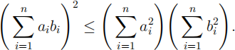
Hint: The Cauchy-Schwarz inequality states that, for numbers a1 , . . . , an and

b1 , . . . , bn ,

Deﬁne the jth random ﬁtted value to be Y(^)j = β(^)LS xj, for j = 1, . . . , n.

(e) Show that

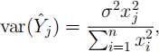
and

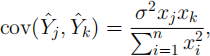
for k = 1, . . . , n. [6 marks]

Hint: For random variables U and V and constants a and b, cov(aU, bV) = abcov(U, V).

2. [Total 28 marks]

(a) Consider a simple linear regression model for the relationship between a response Y and a single explanatory variable x.

(i) State three assumptions that underpin the simple linear regression model. [3 marks]

(ii) After ﬁtting a simple linear regression model to data, describe two diagnostic plots that can be produced and state how the plots should appear if the

assumptions underpinning the model are correct. [4 marks]

(iii) Consider predicting a future observation Y0 with explanatory variable x0 . For ﬁxed observed responses and explanatory variables, what value of x0 will

minimise the width of the 100(1 - Q)% prediction interval for Y0 ? Justify your answer. [3 marks]

(b) The R output below shows the result of ﬁtting a simple linear regression model to data from the 2016 National Football League (NFL) season. For each of the

n = 32 teams, the response is the number of games won (out of 16) in the 2016 season and the explanatory variable is the average number of points scored per game. Additionally, if xi is the average number of points per game for the ith

team, then Σ1 xi = 728.6 and Σni=1 x2i = 17118.44.

## Call:

## lm(formula = wins ~ points)

## Residuals:

## Min 1Q Median 3Q Max

## -4.3954 -1.9349 0.0711 2.0985 4.5602

## Coefficients:

## Estimate Std. Error t value Pr(>|t|)

## (Intercept) -2.1849 2.6811 -0.815 0.421524

## points 0.4446 0.1159 3.835 0.000599 ***

## ---

## Signif. codes: 0 '***' 0.001 '**' 0.01 '*' 0.05 '.' 0.1 ' ' 1

## Residual standard error: 2.666 on 30 degrees of freedom

## Multiple R-squared: 0.329,Adjusted R-squared: 0.3066

## F-statistic: 14.71 on 1 and 30 DF, p-value: 0.0005992

(i) Under the ﬁtted model, what is the estimated increase in expected number of wins per season if average points per game increased by δ? Estimate how many more points a team would need to score on average per game to

increase their expected number of wins per season by one. [4 marks]

(ii) Suppose a team scores an average of 18 points per game. Calculate a 95% prediction interval for the number of games they will win in a season. [7 marks] Hint: You may ﬁnd some of the following R code and output useful

qt(0.975, df = 30)

## [1] 2.042272

qt(0.95, df = 30)

## [1] 1.697261

The NFL is actually split into separate conferences; the American Football

Conference (AFC) and the National Football Conference (NFC), with each team belonging to exactly one of these conferences. A dummy variable called z is

created where for the ith team

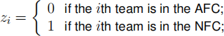
for i = 1, . . . , n.

The R output below shows the result of ﬁtting a further linear regression model to

the data from the 2016 National Football League (NFL) season, this time including the dummy variable.

## Call:

## lm(formula = wins ~ points + z + points * z)

## Residuals:

## Min 1Q Median 3Q Max

## -5.1241 -1.9322 0.2006 1.7199 4.4627

## Coefficients:

## Estimate Std. Error t value Pr(>|t|)

## (Intercept) -6.5646 4.5121 -1.455 0.15682

## points 0.6519 0.1989 3.278 0.00279 **

## z 6.4157 5.6416 1.137 0.26509

## points:z -0.3073 0.2454 -1.252 0.22087

## ---

## Signif. codes: 0 '***' 0.001 '**' 0.01 '*' 0.05 '.' 0.1 ' ' 1

## Residual standard error: 2.671 on 28 degrees of freedom

## Multiple R-squared: 0.3717,Adjusted R-squared: 0.3044

## F-statistic: 5.521 on 3 and 28 DF, p-value: 0.00416

(iii) By considering the above ﬁtted model, write down an expression giving the

estimated expected number of wins per season for AFC teams who score x points per game. Write down the corresponding expression for teams from the NFC. [7 marks]

3. [Total 40 marks]

(a) Suppose n responses Y = (Y1 , . . . , Yn ) satisfy the following general linear regression model

Y = X1β 1 + X2β 2 + ε ,

where ε ~ N (0, σ2In ).

However, the following general linear regression model is ﬁtted Y = X1β 1 + ε ,

where ε ~ N (0, σ2In ).

Show that the bias of the least squares estimator of β1 under the ﬁtted model is equal to

bias(β(^)1 ) = E(β(^)1 ) - β1 = (X1(T)X1 )-1X1(T)X2β 2 . [6 marks]

(b) An experiment has been performed to investigate the relationship between the

heat evolved in the setting of cement and its chemical composition. The

response is the heat evolved and there are m = 3 explanatory variables (x1 , x2 and x3) giving the percentage weight in clinkers of three different chemicals. A total of n = 13 samples of cement were used in the experiment.

A series of eight linear regression models, labelled A, B, . . . , H, are ﬁtted. The table below shows the residual sum of squares (RSS, to 3 decimal places) of each of these models where the + or — in the columns headed x1 , x2 and x3 indicates whether the model includes (+) or excludes (—) the corresponding explanatory variable.

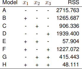
(i) For each model (A, B,. . . ,H), write down the value of k, the number of explanatory variables. [1 mark]

(ii) Consider the use of the Akaike information criterion (AIC) and the Bayesian

information criterion (BIC) for model selection. Explain how both AIC and BIC balance goodness-of-ﬁt and model complexity, remarking on the relative strength of penalties for model complexity of AIC and BIC. [4 marks]

(iii) For each model (A, B,. . . ,H), calculate the value of n log (RSS/n), where

log(·) refers to the natural logarithm. Hence calculate the value of AIC and BIC for each model. [4 marks]

(iv) For each model (A, B,. . . ,H), calculate the value of the corrected Akaike information criterion, given by

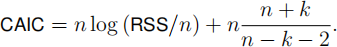[4 marks]

(v) Determine the ﬁnal chosen model under each of AIC, BIC and CAIC. [3 marks]

Below are a series of analysis of variance (ANOVA) tables presenting the result of F-tests. All quantities are given to 3 decimal places.

• Comparison of Model E & Model H

Source	Df	Sum of Squares	Mean Squares	F Value	P Value
Difference	1	9.794	9.794	1.832	0.209
Model H	9	48.111	5.346

Model E

57.904

• Comparison of Model F & Model H

Source	Df	Sum of Squares	Mean Squares	F Value	P Value
Difference	1	1178.961	1178.961	220.547	< 0.001
Model H	9	48.111	5.346

Model F

1227.072

• Comparison of Model G & Model H

Source	Df	Sum of Squares	Mean Squares	F Value	P Value
Difference	1	367.332	367.332	68.716	< 0.001
Model H	9	48.111	5.346

Model G

415.443

• Comparison of Model B & Model E

Source	Df	Sum of Squares	Mean Squares	F Value	P Value
Difference	1	1207.782	1207.782	208.582	< 0.001
Model E	10	57.904	5.790

Model B

1265.687

• Comparison of Model C & Model E

Source	Df	Sum of Squares	Mean Squares	F Value	P Value
Difference	1	848.432	848.432	146.523	< 0.001
Model E	10	57.904	5.790

Model C

906.336

(vi) From the above ANOVA tables, outline the steps taken by a backwards

selection modelselection procedure using F-tests. For each step, name the current model and the models that are compared to the current model. Clearly state the ﬁnal chosen model. Use the 5% level of signiﬁcance. [6 marks]

(vii) Perform a forwards selection modelselection procedure using F-tests. Use the 5% level of signiﬁcance. [12 marks]

Hint: You will ﬁnd the following R code and output useful

qf(0.95, df1 = 1, df2 = 11)

## [1] 4.844336

qf(0.95, df1 = 1, df2 = 10)

## [1] 4.964603