关键词 > MATH2010

MATH2010 Statistical Modelling I SEMESTER 1 EXAMINATION 2021/22

发布时间：2024-06-15

Hello, dear friend, you can consult us at any time if you have any questions, add WeChat: daixieit

MATH2010 Statistical Modelling I

SEMESTER 1 EXAMINATION 2021/22

1. [25 marks] Consider the following simple linear regression model without intercept:

Yi = βxi + ∈i , (1)

i = 1, . . . , n, where ∈i ~ N(0, σ2 ).

(a) [5 marks] Show that the least-squares estimator for β has the form:

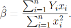
Show thatβ(^) is unbiased, and compute its variance.

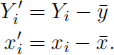
(b) [2 marks] Given explanatory variables x1 , . . . , xn and associated response variables y1 , . . . , yn, it is common to center the response and explanatory variables, i.e. to compute

Consider the alternative model:

YiI = βIxi(I) + ∈i. (2)

Derive the least-squares estimator for βI in terms of xi and Yi.

(c) [2 marks] Explain the difference between an estimator and an estimate. Write down the estimate corresponding to β' from model (2).

(d) [4 marks] Recall that under the simple linear regression model

Yi = β0 + β1xi + ∈i (3)

the estimate for β1 is given by

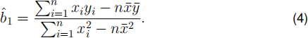
Show that the estimate obtained in (c) is equal to b(^)1 .

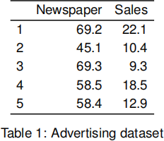
(e) The dataset in Table 1 gives the sales (yi; in £) and the advertising budget spent on newspaper advertisements (xi; in £) for a variety of products.

advertising.data = data.frame(

Newspaper=c(69.2, 45.1, 69.3, 58.5, 58.4),

Sales = c(22.1, 10.4, 9.3, 18.5, 12.9)

)

(i) [8 marks] Compute a 95% conﬁdence interval for β in model (1), and β, in model (2). Test the null hypothesis that β = 0, and the null hypothesis that β, = 0, at the 95% level. You may ﬁnd the following outputs from R helpful:

qt(0.95, 4)

## [1] 2.13

qt(0.95, 3)

## [1] 2.35

qt(0.975, 4)

## [1] 2.78

qt(0.975, 3)

## [1] 3.18

(ii) [4 marks] Consider the location x0 = 0, and let x = x0 - . Let

Y(^)0 = βx0 + ∈0 and Y(^)0, = β,x + ∈0 . Write down the conditional means

E(Y(^)0 ) and E(Y(^)0, ). Considering the computed conditional means, do you think

model (1) or model (2) is more appropriate for this data? Considering the

conﬁdence intervals computed above, do you believe there is a signiﬁcant relationship between budget spent on newspaper advertisements and sales?

2. [25 marks] Consider the usual multiple linear regression model Y = Xβ + ε ,

with Y an n × 1 response vector, X an n × (k + 1) design matrix, β a k + 1 vector of unknown parameters and ε ~ N (0, σ2In ). Assume least squares will be used to estimate β .

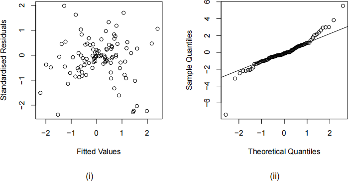
(a) [2 marks] Describe two diagnostic plots that are commonly used to check the assumptions that underpin a linear model, and discuss which assumptions they are intended to verify.

(b) [2 marks] Consider the following two plots. Explain what evidence of deviation from the model assumptions are shown in each plot.

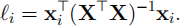
(c) [8 marks] The leverage li of the ith observation is deﬁned to be the derivative of the ith ﬁtted value with-respect-to the ith observation,i.e.:

Show that li is given by

(d) [2 marks] A data point (xi , yi ) is said to be inﬂuential if the regression line

changes signiﬁcantly when that point is excluded from the analysis. There can be more than one inﬂuential point for a regression model. Consider a scatter plot of leverages on the x-axis against standardised residuals on they-axis such as the ﬁgure below.

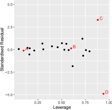
Which of the labelled points on the ﬁgure above do you think could be inﬂuential? Explain why.

(e) Consider the “leave-one-out” procedure, in which observation i is left out of the

regression analysis. Letb(^)(-i) denote the parameter vector obtained when

observation i is left out, and recall that we have the following formula for the change in the parameter vector:

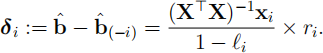
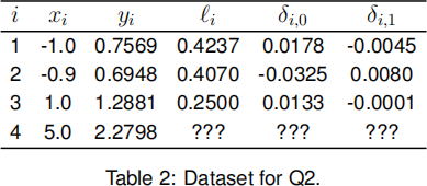
where ri is the ith residual, ri = yi - ^(y)i. Consider the simple linear regression problem Yi = β0 + β1xi + ∈i. In this case, δ i is a vector of length 2,

δ i = [δi;0, δi;1]. The dataset in Table 2 gives 4 observations of the response yi , with explanatory variable xi, as well as the values of li and δi for all but the 4th observation.

The data can be read into R with the command:

data = data.frame(

x = c(-1, -0.9, 1, 5),

y = c(0.7569, 0.6948, 1.2881, 2.2798)

)

(i) [8 marks] Compute l4 , δ4;0 and δ4;1 . If you use R, or other software, to answer this question, please clearly state the commands you use.

(ii) [3 marks] Do you think the fourth point is more inﬂuential than the ﬁrst three points? Explain why, or why not, particularly commenting on the values of l4 , δ4;0 and δ4;1 in your answer.

3. [25 marks] In a particular data set, n = 20 observations were made on a response variable (y) and three explanatory variables (x1, x2 and x3).

(a) [6 marks] Partial outputs from the summary command in R applied to lm objects regressing each of the explanatory variables on the response separately are given below. From this output, calculate AIC for each of the three models.

## Call:

## lm(formula = y ~ x1)

## Coefficients:

## Estimate Std. Error t value Pr(>|t|)

## (Intercept) 13.3004 0.5331 24.95 2.1e-15

## x1 0.0989 0.5857 0.17 0.87

## Residual standard error: 2.33 on 18 degrees of freedom

## F-statistic: 0.0285 on 1 and 18 DF, p-value: 0.868

## Call:

## lm(formula = y ~ x2)

## Coefficients:

## Estimate Std. Error t value Pr(>|t|)

## (Intercept) 13.334 0.262 50.96 < 2e-16

## x2 2.255 0.308 7.32 8.5e-07

## Residual standard error: 1.17 on 18 degrees of freedom

## F-statistic: 53.6 on 1 and 18 DF, p-value: 8.51e-07

## Call:

## lm(formula = y ~ x3)

## Coefficients:

## Estimate Std. Error t value Pr(>|t|)

## (Intercept) 13.302 0.250 53.18 < 2e-16

## x3 2.339 0.301 7.77 3.7e-07

## Residual standard error: 1.12 on 18 degrees of freedom

## F-statistic: 60.3 on 1 and 18 DF, p-value: 3.73e-07

(b) [2 marks] Given that AIC for the null model (containing no explanatory variables) is 31.783, which is the ﬁrst variable that you would include when building a model using forward selection and AIC?

ﬁtted using lm, and partial output from the summary command is given below.

## Call:

## lm(formula = y ~ x1 + x2 + x3)

## Coefficients:

## Estimate Std. Error t value Pr(>|t|)

## (Intercept) 13.186 0.244 54.09 <2e-16

## x1 0.515 0.281 1.83 0.086

## x2 -1.192 3.171 -0.38 0.712

## x3 3.660 3.227 1.13 0.273

## Residual standard error: 1.06 on 16 degrees of freedom

Using t-tests, which variables can be individually dropped from the model without adversely affecting the quality of the ﬁt?

(d) [5 marks] Give a possible explanation for the contradiction between your results from parts (b) and (c).

(e) [4 marks] Given that the sample variance of the response is sy(2) = 5.157, what is

the adjusted R2 value for the above multiple regression model? Is the model a good ﬁt?

(f) [6 marks] Test the signiﬁcance of the multiple regression model for these data; that is, compare it to the null model.

You may ﬁnd the following quantities from R useful:

qf(0.95, 4, 16)

## [1] 3.01

qf(0.95, 3, 16)

## [1] 3.24

qf(0.95, 3, 20)

## [1] 3.1

4. [25 marks] Every year Forbes produces a data set of the top 2000 companies

world-wide, ranked by quantities such as Sales and Assets, across different market sectors, countries etc.

A linear model was ﬁtted to the 2017 data, regressing log(Sales) against

log(Assets) (aquantitative variable) and Sector (a qualitative factor with 11 levels). The following analysis of variance table was obtained.

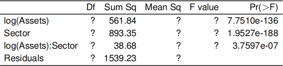
(a) [6 marks] Write down each of the nested model comparisons summarised in this table.

(b) [8 marks] Complete the ANOVA table. Give reasons for your choices for each entry in the “DF” column.

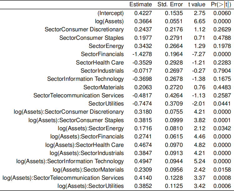
(d) [10 marks] Simpliﬁed output from the summary command from the ﬁtted lm

object in R for this model is given on the next page. The units of each of Sales and Assets are billions of dollars; in the data set, Apple had sales of 217.5 and assets of 331.1, both in billions of dollars, larger than any other “Information

Technology” company.

What is the equation for the estimated mean response (log(Sales)) from a company in the “Information Technology” sector in terms of log(Assets)? What is it for the “Consumer Discretionary” Sector? Sketch a plot with these two equations. At what value of Assets is an information technology company predicted to have greater mean sales than a company in the consumer discretionary sector?

The company with largest sales in the data set is Wal-Mart (a consumer discretionary company), with sales of 485.3. According to the regression model, how large would Apple’s assets need to be to surpass Wal-Mart’s sales? What caveats do you have about this prediction?

Learning objectives:

LO1 Use the theory of linear models and matrix algebra to investigate standard and non- standard problems.

LO2 Interpret the output from an analysis including the meaning of interactions and terms based on qualitative factors.

LO3 Understand how to make a critical appraisal of a ﬁtted model.

LO4 Carry out t-tests and calculate conﬁdence intervals by hand and by computer. LO5 Using a variety of procedures for variable selection.

LO6 Fit multiple regression models using the adopted software package.

LO7 Carry out simple linear regression by computer.

LO6 and LO7 are assessed via coursework.