关键词 > MATH2010
MATH2010 Statistical Modelling I SEMESTER 2 EXAMINATION 2022/23
发布时间:2024-06-15
Hello, dear friend, you can consult us at any time if you have any questions, add WeChat: daixieit
MATH2010 Statistical Modelling I
SEMESTER 2 EXAMINATION 2022/23
1. [Total of 30 marks]
(a) [Total of 15 marks] Consider the multiple regression model
where Yi is the response variable, the xij are the observed values of explanatory
variables and ϵi iid ∼ N(0, σ2).
(i) [5 marks] Show how this model can be expressed in the form Y = Xβ + ϵ
stating clearly the distributions of both the random vectors Y and ϵ . (ii) [2 marks] Describe three assumptions that underlie a multiple linear regression model.
(iii) [3 marks] Describe two diagnostic plots that could be used to verify these
assumptions. Sketch how those plots might appear: i. If the model is adequate.
ii. If the residuals are long-tailed (also sometimes referred to as heavy-tailed). iii. In the presence of heteroscedasticity.
(iv) [5 marks] Define the hat matrix H and give expressions for estimators for the
fitted values Y(ˆ) and residuals R in terms of H. Show that Cov(Y(ˆ) , R) = 0, stating any properties of the hat matrix that you use. Comment on the significance of this for interpreting the diagnostic plots described above.
(b) [Total of 15 marks] A random sample of 9 auction prices (Y, in dollars) of
grandfather clocks (a type of antique clock), along with the clock age (x1 , in
years) and the number of bidders (x2) was recorded. The data are given below:
age = c(132, 174, 142, 182, 186, 111, 152, 182, 154)
bidders = c(14, 9, 11, 10, 6, 13, 7, 5, 8)
price = c(1537, 1501, 1292, 1648, 1267, 1275, 1085, 946, 1221)
If you use R to answer any part of this question please clearly state which commands you used.
(i) [2 marks] Fit a multiple linear regression model with the response and explanatory variables given above.
(ii) [1 mark] Perform a test to identify which coefficients are significant at a 1% level of significance.
(iii) [2 marks] Construct a 95% confidence interval for β1 , the coefficient associated with age.
(iv) [1 mark] Perform a hypothesis test for the null hypothesis H0 : β1 = 10 at the 5% level.
(v) [5 marks] Another clock was sold, with age=200 and bidders=10. Produce 90% confidence and prediction intervals for the price of this clock. Explain the difference in width between the two intervals. Can you identify any problems that might be associated with this prediction?
(vi) [4 marks] Provide a practical interpretation of the estimated intercept. Can you see any problem with this interpretation? If so, suggest a transformation of the model that might address this. (Note: You do not need to fit the transformed model.)
2. [Total of 25 marks] Consider the following regression model:
Y = Xβ + ϵ , (1)
where Y is then-dimensional vector of response variables. X is then × pmatrix of explanatory variables, β is the p-vector of parameters and ϵ is a n-dimensional
vector valued random variable with components ϵi iid ∼ N(0, σ2)
(a) [6 marks] Show that the least-squares estimator for β is given by
β(ˆ)LS = (XTX)—1X TY
and derive its sampling distribution.
Consider all linear estimators of β, that is, all estimators that are of the form
β(ˆ)W = WY
with W an p × nmatrix.
(b) [4 marks] Compute E(β(ˆ)W ), and show that its variance is Var(β(ˆ)W ) = σ 2 WW T.
(c) [2 marks] Show that β(ˆ)W is unbiased if and only if WX = I.
(d) [10 marks] Let
E := Var(β(ˆ)W ) — Var(β(ˆ)LS ).
Show that if β(ˆ)W is unbiased then there exists a p × n matrix L such that
E = σ 2 LLT. Hence show that, for any p-dimensional vector w, wT Ew ≥ 0. Hint: it maybe helpful to express the matrix W as W = (XTX)—1XT + L.
(e) [3 marks] For two p-dimensional random vectors Z , Z/, we say that Var(Z) is larger than Var(Z/ ) (written Var(Z) ≥ Var(Z/ )) if
wT Var(Z)w ≥ wT Var(Z/ )w
for all p-dimensional vectors w.
Show that if β(ˆ)W is unbiased then Var(β(ˆ)W ) ≥ Var(β(ˆ)LS ). What does this tell you about the sampling distribution of β(ˆ)LS?
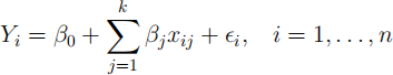
3. [Total of 20 marks] Consider the multiple regression model
Yi = β0 + β1xi1 + β2xi2 + ϵi , i = 1, . . . , n
Where xi1 , xi2 are the observed values of explanatory variables and ϵi iid ∼ N(0, σ2 ).
(a) [5 marks] Express the entries of the matrix X⊤X in terms of xi1 , xi2 and any constants.
(b) [10 marks] Recall that the least-squares estimate of β is
β(ˆ)LS = (X⊤X)−1X ⊤Y .
Suppose that Σni=1 xi2 = 0 and Σni=1 xi1xi2 = 0. Show that the resulting
least-squares estimates of the componentsβ(ˆ)0 , β(ˆ)1 and β(ˆ)2 are β(ˆ)0 = Y(¯) − β(ˆ)1 ¯(x)1
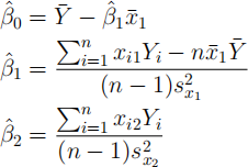
where¯(x)1 and sx(2)1 are the the sample mean and variance of x11 , . . . , xn1 and sx(2)2 is the sample variance of x12 , . . . , xn2 .
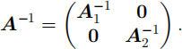
Hint: You may use without proof that if A1 isn1 × n1 and A2 isn2 × n2 , while A is (n1 + n2 ) × (n1 + n2 ) with
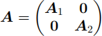
then
(c) [Total of 5 marks] The model above was fitted using R and the model summary is printed on the next page. This has some missing values, indicated by NA.
##
## Call:
## lm(formula = y ~ x_1 + x_2)
##
##
## Coefficients:
## Estimate Std. Error t value Pr(>|t|)
## (Intercept) 0.1864 0.1067 NA NA
## x_1 2.1534 0.1084 NA NA
## x_2 0.2134 0.0963 NA NA
##
## Residual standard error: 0.559 on 31 degrees of freedom
## F-statistic: 165 on 2 and 31 DF, p-value: <2e-16
(i) [1 mark] How many observations were made?
(ii) [4 marks] Fill in the missing values from the output (under “t value” and “Pr(>|t|)”). Which of the variables could be removed without significantly worsening the fit of the model? If you use R to answer this part of the question, please clearly state the commands used.
4. [Total of 25 marks]
The following table summarises model fits for all possible combinations of 3
explanatory variables, x1 , x2 and x3 , based on n = 20 observations. An × in the column indicates that this variable was included in the analysis, a − indicates that it was not.
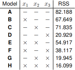
The obtained values of RSS can be loaded into R with the following command:
rss = c (82 . 188, 67 . 649, 71 . 835, 20 . 929, 54 . 917, 38 . 117, 19 . 945, 16 . 099)
If you use R to answer any part of this question, please clearly state the commands used.
(a) [2 marks] For each model, state the number of explanatory variables, the length of the parameter vector β, and the number of degrees of freedom.
(b) [6 marks] For each of the following pairs of models, either perform an F-test
comparing the two models at the 5% significance level, or explain why such a test cannot be performed.
(i) H and E. (ii) H and D. (iii) G and F.
(c) [1 mark] Explain why the residual sum of squares cannot be used for model selection.
(d) [4 marks] For each model,compute AIC and BIC, and identify the best model according to each criterion.
(e) [4 marks] For both forward and backwardselection with AIC:
(i) In each case, what is the final model chosen?
(ii) In each case, for which models would you not need to calculate AIC?
A new factor variable x4 is introduced into the analysis, with three levels labelled 1, 2 and 3. Of the 20 examples in the dataset, n1 were found to be factor 1, n2 were
factor 2 and n3 were factor 3,with n1 + n2 + n3 = 20. The Yi were ordered so that
the first Y1 ,..., Yn1 are factor 1, Yn1 +1,..., Yn1 +n2 are factor 2 and Yn1 +n2 +1 , . . . , Yn are factor 3.
(f) [3 marks] Explain how we would add columns to the design matrix X used in model H to include x4 in the analysis. Describe a constraint that must be introduced to ensure that the new design matrix is nonsingular.
(g) [5 marks] The RSS of the model with x4 included is 15.011. Compare the new model to model H by performing an F-test at the 5% significance level.
Learning objectives:
LO1 Use the theory of linear models and matrix algebra to investigate standard and non- standard problems.
LO2 Interpret the output from an analysis including the meaning of interactions and terms based on qualitative factors.
LO3 Understand how to make a critical appraisal of a fitted model.
LO4 Carry out t-tests and calculate confidence intervals by hand and by computer.
LO5 Using a variety of procedures for variable selection.
LO6 Fit multiple regression models using the adopted software package.
LO7 Carry out simple linear regression by computer.
LO6 and LO7 are assessed via coursework.
