Physics 111L Laboratory Report

Hello, dear friend, you can consult us at any time if you have any questions, add WeChat: daixieit

Physics 111L Laboratory Report

Course Name/Section: Phys 111L/A

Lab Number/Name: Lab 01 / Measurement and Uncertainties

Date: 8/16/2015

Introduction

In this week’s lab we will be learning about measurement error. Our experiment will consist of dropping a mass from known heights and measuring the time it takes the mass to fall. From this, we can calculate the local acceleration of gravity for the falling mass using:

where h is the distance the object falls (in meters), t is the amount of time it falls (in seconds), and g is the local gravitational acceleration constant (m/s2 ). We will consider the uncertainty in our timing measurement, as well as the uncertainty in the height from which the mass is dropped, and use these to determine the error in our calculation of the gravitational acceleration constant. Our results will be compared to the expected value, g = 9.80 m/s2 .

Experimental Procedure

We taped our 2-meter stick to the table with the 0 cm end at the floor. The stick appeared to be straight up and down, though we did not verify this with a plumb-bob. We took measurements from two different heights, 1.50 m and 2.00 m. For each height, the ball bearing was held next to the meter stick such that the bottom of the bearing was lined up with the appropriate height marking on the meter stick. The ball bearing was dropped, and a stopwatch was used to time its fall. The right-handed person dropping the bearing (left hand) also started the stopwatch at the time of release (right hand). They then stopped the stopwatch upon seeing/hearing the bearing strike the floor. We used a piece of cardboard under the meter stick/drop area so as not to damage the floor wax. Each group member (C.D. and Eric) did 10 separate trials at each height.

List of Equipment

1) 2 Meter stick (a stick that was 2 meters long)

2) Tape to secure the meter stick

3) Steel ball bearing

4) Stop watch (1/100 s precision)

Raw Data with Error Estimates

We only considered random error in our experiment (instead of random and systematic error). To estimate the uncertainty in our height measurements, we used the direct method. The meter stick we used had markings at 1 mm. The standard estimate for uncertainty would then be ±0.5 mm (one half of the smallest graduation on our measuring device), but based on the difficulty we had holding the ball bearing in the proper position before release, this uncertainty estimate would be too small. Instead, we approximated the uncertainty in our height measurement to be ±1 cm, or ±0.01 m.

To estimate the error in our timing measurement, we used the statistical method. For the 10 trials at each height, we calculated the average and standard deviation using Excel with the built-in functions AVERAGE and STDEV. The standard error, which is what we use as error in our measurement, is the standard deviation divided by the square root of the number of trials. We did 10 trials for both experiments, so our standard error in each data set was calculated using

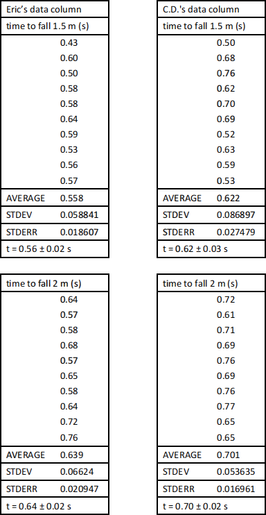
Our time data (and the computed uncertainties) are included Table 1.

Table 1: Data obtained by two different experimenters (Jack and C.D.) dropping a mass from two different heights (1.50 ± 0.01 m and 2.00 ± 0.01 m).

Analysis: Calculations/Error Propagation/Plots

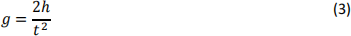
In order to determine the local gravitational acceleration constant, we solve Eq. (1) for g:

Using Eq. (3) and our results from Appendix A we calculate four values of g (and the associated uncertainties) using our data. Calculation of g is straightforward, but the calculation of its uncertainty, Δg, is a little more complicated. We follow the procedure outlined by Eqs. (5) and (6) of the Error Analysis Reference handout. We present only one of the calculations here (Eric’s data for dropping a mass from a 1.50 ± 0.01 m height). For the value of g:

For the uncertainty of this value we must find the deviations due to the uncertainties in h and t:

Note that we used several significant figures for our time average and associated uncertainty to minimize round-off error. We then calculate the uncertainty in g by adding the individual deviations in quadrature:

Lastly, we round our result to the correct number of significant figures to get

We use Eq. (7) of the Error Analysis Reference handout to compare this result to the expected value of , and find the percent error to be:

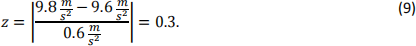
We use Eq. (9) if the Error Analysis Reference handout to determine that the relative uncertainty for this result is:

We must calculate a “z-value” to determine if our measured value, with its uncertainty, is consistent with the accepted value. We use Eq. (10) if the Error Analysis Reference handout calculate z:

These calculations where repeated for each of the other three data sets.

Results with Error Estimates

To decide if our measured value is consistent with the expect value of , we use Eqs. (11) of the Error Analysis Reference handout, which just says that the z-value for the measured value must be less than 2 to be considered consistent. The z-value for the case shown in the previous section is less than 2, and therefore that measurement is consistent with the expected value.

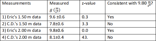
Our results are summaries in Table 2.

Table 2: Our results for four individual measurements of local gravitational acceleration.

Answers to Lab Questions

1) Compare your data with that of your partner for the 1.5 m fall heights. Are they consistent with one another (use Eq. (12) of the Error Analysis Reference handout to determine this)? Also do a similar comparison for the 2.0 m fall height data.

ANSWER

Eric and C.D’s 1.5 m data comparison: because 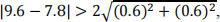it is clear that the measurements are not consistent with one another.

Eric and C.D’s 2.0 m data comparison: because it is again clear that the measurements are not consistent with one an other.

2) If you found that some of your measured results are inconsistent with the expected value of g, come up at least two possible reasons for the discrepancy.

ANSWER

Eric’s data are consistent with the expected value, but C.D’s aren’t. This implies that C.D.’s data collection procedure was flawed in some way. In this experiment, it is very difficult to correctly acquire timing data, due to human reaction time (~0.2 s). It is also very hard to determine if the experimenter actually sees or hears the bearing strike the ground before or after the stop watch has been stopped. Air resistance and the speed of sound are also possible problems, although in this case their effects are minor. Ultimately, this is a poorly designed experiment and it would be better to time several oscillations of an oscillating pendulum to perform a measurement of g.

3) Explain how you could make the uncertainties in your measurments even smaller.

ANSWER

Collecting more data should make the uncertainties smaller, as the standard error of the mean decrease as

4) What do you think the effect of the mass of the dropped sphere has to do with this experiment, i.e. what would have been different if you had used a sphere with a different mass? Explain.

ANSWER

Since mass does not appear in Eqs. (1) or (3), there should be no mass dependence, i.e. doing the experiment with a sphere of different mass should not appreciably change the results. This is in agreement with Giambattista Benedetti’s early experiments (~1553).