MGT001371 - Scheduling Manufacturing Systems Homework Assignment II

发布时间：2024-06-07

Hello, dear friend, you can consult us at any time if you have any questions, add WeChat: daixieit

MGT001371 - Scheduling Manufacturing Systems

Homework Assignment II

• To be submitted on 13.06.2024 (Thursday 13:00) via TUM Moodle.

• Late submission will not be accepted. No collaboration!

• You must submit your handwritten or typewritten solutions in a single .pdf file and your codes in separate .py files.

• You should zip (compress) all of your files and name the .zip file as ”NameLast- name studentID”, i.e., ”BaharOkumusoglu 01234567.zip” .

• Coding questions will be graded based on the result they generate and not the entire syntax. If a particular code section does not work, zero points are given to that section. We try to give points for the outcome of individual code sections wherever possible but reserve the right to grade multiple sections together if necessary.

• Be precise. Do not make vague statements and leave any room for interpretation. You must also present your step-by-step solutions wherever applicable.

1. (10 points) Consider a car manufacturing company that operates a paced assembly line. Let us denote the sets of models, options and parts as M, O and P, respectively. The company can produce model m ∈ M with option o ∈ O and part p ∈ P. We also define the set of production cycles and the set of stations at the production line as T and K, respectively. Suppose the company wants to determine the sequencing for its production line to avoid work overloads by solving different optimization problems. The problem parameters and decision variables are provided in Table 1.

Implement the following optimization models using the Python-Gurobi interface with the provided data using the code template Sequencing Template .py. For each model, you need to write a function and call this function to get the optimal sequencing decisions. To avoid code repetitions, you should call the function BaseModel whenever required. Also, recall that variable indexing in Python starts from 0.

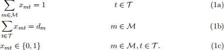
(a) (3 points) (Base Model) The function in your code should take a Gurobi model object as an argument and add the following constraints:

Parameters

dm Demand for copies of model m.

c Cycle time.

lk Length of station k.

pmk Processing time of model m at station k.

amo 1, if model m requires option o, and 0 otherwise.

pmo Demand of model m for part p.

rcp Target consumption rate of part p.

rcm Target production rate of model m.

Decision Variables

xmt 1 if model m is produced in cycle t, and 0 otherwise.

wkt Work overload occurring at station k in cycle t.

skt Start position of the worker at station k when cycle t begins.

ymt Total cumulative production quantity (in integer) of model m up to cycle t.

Table 1: Problem parameters and decision variables.

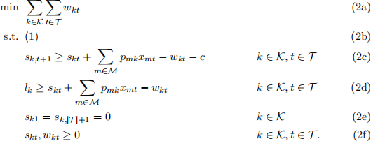
(b) (3 points) (Mixed-model Sequencing Model)

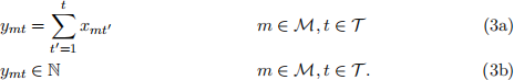
(c) (4 points) (Level-scheduling Model) Your function should take a flag as an argu- ment and use it in a conditional statement in order to solve the problem for part-oriented and model-oriented versions. Your function should create an optimization model with the following objective functions

for the part-oriented and the model-oriented models, respectively. Note that the feasible regions for both models are defined by (1) and the following set of constraints:

Hint: When defining a quadratic objective in the solver, you cannot use the expression x2 , instead, you should use x ∗ x. As a rule of thumb, always use parentheses when there are summations for the quadratic expressions, i.e., Σi(xi) ∗ (xi).

2. (4 points) Consider the economic lot sizing problem with several items on a single machine under the sequence-independence assumption. Using the provided data with the code tem- plate ELS Template .py:

(a) (2 points) write a function basicESL that returns the cycle time, idle time, production run and maximum inventory for each item.

(b) (2 points) provide a detailed inventory level chart by indicating the necessary points at the chart.

3. (12 points) The capacitated lot-sizing problem with zero setup times can be formulated as a mixed-integer programming problem. Let N and T be the sets of items and periods, respectively. The problem parameters and decisions variables are given as follows:

Parameters

dit Deterministic demand for item i in period t.

P(¯) Production capacity for machine.

vit Production rate product i in period t.

hit Holding cost for item i in period t.

cit Setup cost for item i in period t.

Ii0 Initial inventory for item i.

Decision Variables

Iit Inventory for item i at the end of period t.

xit Production amount for item i in period t.

yit 1, if machine is setup for item i in period t, 0 otherwise.

zit 1, if item i is produced in period t, 0 otherwise.

Table 2: Problem parameters and decision variables.

Implement the following optimization models using Python-Gurobi interface with the pro- vided data with the code template ESL Template .py. For each model, you are supposed to use only one function ESLModel and call this function to get the optimal solutions. You should include conditional statements in this function such that some part of the function will run depending on the optimization model given by the following parts. For exam-ple, when you want to solve the optimization model (4), you should include a conditional statement if modelType == ‘bigBucket’ such that your function will ONLY create the optimization model for this model.

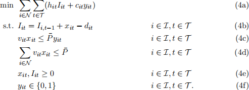
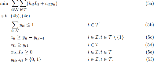
(a) (5 points) (Base Model, Big Bucket)

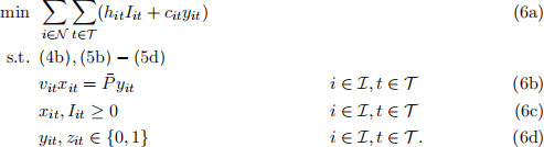
(b) (3 points) (Small Bucket, Continuous)

(c) (4 points) (Small Bucket, Discrete) In your function, you should not rewrite con- straint (6b) as it is. Instead, you should only add a single constraint that implies constraint (6b).

4. (4 points) Consider the robust sequencing problem discussed in class. In the optimization model, there are some nonlinearities due to the constraints corresponding to the number of violations per option in failure scenarios and the length of evaluation windows. Also, see ”Robust car sequencing for automotive assembly, A. Hottenrott, L. Waidner, M. Grunow, EJOR (2020)” .

(a) (1 point) Indicate and discuss the nonlinearities induced by these constraints.

(b) (3 points) For ease of notation, consider the following two constraints corresponding to the number of violations per option in failure scenarios and the length of evaluation windows:

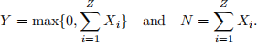
Here, the decision variables are X ∈ {0, 1}, Y ∈ N, Z ∈ Z+ and N ∈ N. Moreover, assume that the decision variable Z has a finite upper bound Z(¯) . Linearize these con-straints by introducing auxiliary variables. Show your step-by-step solutions and write your final system of equations in the box below. (Hint: First linearize the second con-straint by introducing Z(¯) many binary decision variables and replace the domain of the summation by (1, Z(¯)). Then, rewrite constraint by coupling these new variables and X variables. You should introduce more auxiliary variables in the rest of the exercise.)