关键词 > 4035
4035 Communications IV MATLAB Assignment
发布时间:2024-06-04
Hello, dear friend, you can consult us at any time if you have any questions, add WeChat: daixieit
4035 Communications IV
MATLAB Assignment – 10% of Final Assessment
The assignment is to generate a frequency modulated signal, add noise, filter and demodulate it, and hence calculate the signal to noise ratio. The RF signal will be generated and demodulated in phasor form (ie. the carrier modulation operation will not be done). The output signal component will be determined by correlating the output signal with the output signal under noise free conditions.
Specified Parameters
|
Baseband bandwidth |
W |
15 kHz |
|
RF carrier amplitude |
A |
1 V (peak) |
|
Frequency deviation |
fd |
75 kHz |
|
Noise spectral density |
No |
such that Pr/NoW = A2/2NoW = 10 dB to 30 dB in steps of 1 dB. |
|
Sampling frequency |
fs |
360 kHz |
|
Number of samples |
N |
100,000 |
All signals will be represented in sampled form with a sampling interval Δ = 1/fs. To avoid numerical ill- conditioning, it is recommended that you use frequencies in units of MHz rather than Hz (ie fs = 0.360, W = 0.015, etc), and this will give Δ in units of μsec.
1. Modulating Signal
Two modulating signals will be used, both such that |m(t)| ≤ 1.
a) Sinewave of frequency 2 KHz.
m(t) = sin(2π 2000t)
b) Random Signal.
The second will be a random signal generated by filtering Gaussian white noise and normalised to |m(t)| ≤ 1. The signal is generated by generating independent Gaussian samples and filtering them using a digital filter H1 of 3 dB bandwidth 2 kHz. The design of this filter is based on a single pole analog filter:
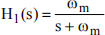
where ωm is the 3 dB bandwidth of the analog filter in radians/sec (in scaled form this will be in Mrad/sec).
This signal is then bandlimited by filtering with a digital filter H2 of 3 dB bandwidth 15 kHz. The design of this filter is based on a fifth order analog Butterworth filter:

where ωc is the 3 dB bandwidth of the analog filter in radians/sec (in scaled form this will be in Mrad/sec). The digital filters should be realised using the bilinear transformation (where Δ = 1/fs):

This leads to a “frequency warping” such that the response of the digital filter is the same as that of the analog filter but the frequency scales are related by the relation:
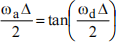
where ωa is the frequency in the analog filter and ωd is the frequency in the digital filter. Since it is ωd which is specified as the 3 dB bandwidth, you need to calculate the appropriate value of ωa and then apply the bilinear transformation.
Matlab has a routine bilinear, which will do the bilinear transformation for you, but make sure you use it correctly. It will even do the frequency warping for you if you set the parameters correctly.
You first need to generate this signal using Gaussian random noise samples of unity variance (the function randn is recommended), filter these with H1 and H2 and then scale the filtered output so that it does not exceed the values ±1. All filtering operations can be carried out with the Matlab function filter.
2. The Receiver Filters
Carson’s rule gives a required RF bandwidth of B = 2(fd+W) = 180 kHz. However because we are using a phasor (equivalent baseband) representation, the filter H3 for the phasor is low pass of bandwidth 90 kHz. The sampling frequency chosen is four times this. The filter H3 is a digital fifth order Butterworth filter, and can be realised in digital form in a similar manner to H2. The post-detection filter H4 will be the same as H2 and is of 15 kHz bandwidth. As before, all filtering operations can be carried out with the Matlab function filter.
If we include modulation onto an RF carrier frequency, the sampling frequency would have to be at least twice the carrier frequency and this would slow the simulation significantly. For that reason we do all the simulation of RF signals using phasors.
3. Modulation
The FM signal as received is of the form:
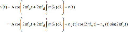
In phasor form this is:
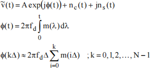
[Note that Matlab indices start at 1, not 0].
4. Additive Noise
The noise added to the RF signal is n(t) of power spectral density Snn(f) = No/2. The noise phasor is)t(jn)t(n)t(. The real and imaginary parts both have a spectral density of No, and in sampled form these are realised as independent Gaussian noise samples of variance σ2 = Nofs. The value of No can be calculated from the value of Pr/NoW.
5. Demodulation
Demodulation is achieved by calculating the instantaneous phase θ(t) of the predetection signal (which is simply the angle of the phasor). To avoid phase discontinuities, you should use the unwrap function in Matlab. The instantaneous frequency is then found by differentiation,
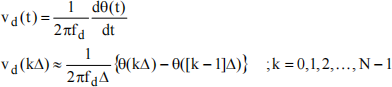
[Assume θ(−1) = 0]. This will give vd(t) = m(t) if θ(t) = φ(t) which should be very nearly so under noise free conditions (filtering an FM signal does cause some non-linear distortion in the modulation).
6. Postdetection Filtering
The signal vd(t) is then filtered with H4 to give the output signal vo(t). The output SNR formula derived in lectures assumes an ideal post-detection filter. In the simulation a 5th order Butterworth filter is used, and for this the noise output is 1.1530 times larger than with an ideal filter. You should take this factor into account when calculating the theoretical output SNR, and you should get good agreement with your simulation (above threshold).
For recovery of the signal and noise it is necessary to generate a reference signal v ref(t) which is the value of vo(t) with no added noise. Generate the reference signal before the actual simulation begins, and ensure the same m(t) is used for the reference and each simulation.
7. Separation of Signal and Noise
We assume the output signal is of the form:
vo (t) = so (t) + n o (t) = λ v ref(t) + n o (t)
We then correlate this with vref(t) to form:
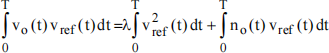
We now assume that the second integral is approximately zero (because the signal and noise are uncorrelated), and this then gives us an estimate for λ and hence the signal and noise components of the output.
In Matlab, of course, the integrals are approximated by summations. You can now calculate the output signal and noise powers and hence the output signal to noise ratio in decibels. A large number of samples is required if this is to be accurate, and that is why we use N = 100,000.
8. Simulation
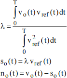
The FM system will be simulated so that the RF & IF signals are represented in equivalent low pass form (ie. the phasor representation of RF and IF signals will be used). The actual RF & IF signals will not be used. The structure of the simulation is shown below.
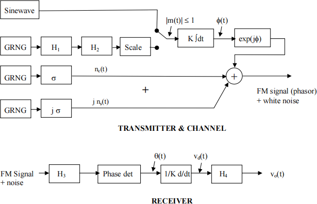
GRNG = Gaussian Random Number Generator, zero mean and unity variance (randn is recommended).
σ = variance of noise sample
At the receiver, the first filter H3 represents the pre-detection RF and IF filters. Note that in phasor form the input and output of this filter are both complex (which is no problem forMatlab). The filter H4 filter is the post-detection filter and its input and output are both real.
9. Tasks to be Performed
The emphasis in this assignment is to attempt a working simulation and does not require extensive use of Matlab functions or fancy programming. However, if you use “high level” Matlab functions, make sure you understand precisely what they do and set the parameters to appropriate values. It is often more straightforward to use simple functions.
Obviously a good working simulation will attract marks. But at the end of the day, I’m looking for a well structured methodology and evidence that you had an exploratory attitude to the problem. I don’t want to just see a neat solution; I want to see you take “ownership” of the assignment by describing your exploratory steps to arriving at your final code. For example, you may want make intermediate plots to convince yourself individual parts of your code are working, you may want to plot relevant formulas and functions to test how they behave. You may want to generate some trial plots that test how the random number generator behaves or how phase unwrapping behaves (for example) and so on. You are encouraged to put your investigations and “sanity check” plots into your report to show you really owned this assignment.
If you mess up the assignment it is still possible to get reasonable marks, if you diligently show the steps you took to gain ownership and the steps you took to explore the problem space.
Your submission should contain a detailed description of your procedures, any theoretical analysis necessary, the graphical plots specified, and your MATLAB code with plenty of comments. The assignment is expected to be your own work, copies of another person's work will not be favourably received and you should carefully note the policy on plagiarism.
• Rule 1: The top caption of every Matlab graph must contain your Student ID and name.
• Rule 2: You must submit fully commented Matlab code with your assignment. The header for each code module should contain a comment with your name, date, and student ID.
• Rule 3: As well as a hard copy, you must attach a CD pouch to your report and insert a CD of your whole project directory containing all the Matlab files, log files, Word files, pdf files, and any files relating to this assignment.
• Rule 4: Submit the assigment in the assignment box. Do not submit to me or anyone else. If you submit late, you must hand it into the Departmental office and ask for it to be date & time stamped. Late ubmissions without a stamp will receive zero marks.
• Rule 5: The assigment must be handed up together with a signed cover sheet.
• Rule 6: Any slightest violation of Rules 1-5 will receive zero marks.
In order to get repeatable results, you should set the seed of the Gaussian random number generator once only at the beginning of your simulation. You can try different seeds and see if the results differ, but in what follows you need only show the results for one seed.
1. Plot the magnitude of the frequency responses of H1, H2 and H3 in dB and show clearly that the correct 3 dB frequencies are realised. Only show the response from −30 dB to +5 dB and a frequency scale of 0 to 180 kHz.
The following tasks 2−8 are to be carried out first with sinusoidal modulation and then with the random modulation signal.
2. Generate the message signal m(t).
3. Generate the reference signal v ref(t).
4. Generate the random numbers (with unit variance) to be used for nc(t) and ns(t).
5. For each value of Pr/NoW scale the noise phasors to the correct variance, run the simulation and calculate the output signal to noise ratio in dB.
6. For Pr/NoW = 17 dB only, plot so(t) and no(t) for 0 ≤ t ≤ 10 ms.
7. Plot the output signal to noise ratio in dB against Pr/NoW in decibels. From a calculated value of
discussed in Section 6.
8. Estimate from your simulation the predetection signal to noise ratio at which threshold occurs (for both types of modulation). A reasonable definition of the threshold point is where the output signal to noise ratio is about 1 dB worse than the theoretical value.
Comment briefly on the significance of your results.
