Maths 787 Special Topic: Inverse Problems and Stochastic Differential Equations Assignment 3

Hello, dear friend, you can consult us at any time if you have any questions, add WeChat: daixieit

Maths 787 Special Topic: Inverse Problems and Stochastic Differential Equations

Assignment 3, due by 3 pm on Friday, 31 May, 2024

Consider the Fredholm integral

with the kernel function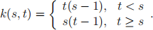

Q1. Analysing the kernel operator

(a) Let ˆx(t) be the second derivative of x, i.e., 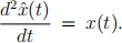Show, by twice partial integration of (1), that

(b) Show that

Take x(t) ≡ 1, for all t in [0, 1], and compute the data y(t). Similarly, compute y(t) for x(t) = t, for all t in [0, 1]. Are both data y(t) in the range of K?

Hint: y ∈ H2 ([0, 1]) means that y is twice differentiable and y, y' and y'' are L2 ([0, 1]).

(c) Linear operator K : L2 ([0, 1]) → L2 ([0, 1]) is self-adjoint, i.e., K∗ = K. Show that reg-ularised solutions ˆx(t) also fulfil ˆx(0) = ˆx(1) = 0 and are twice differentiable. Explain how regularised solutions may never be the original parameter x.

Hint: Check the examples from (b).

Q2. Solving the linear inverse problem

The kernel operator has been discretised on a meshgrid with mesh size 10−3 , i.e., 1001 to describe the interval [0, 1]. The resulting 1001 × 1001 matrix K is given in file Kernel.mat. You may check that K is a singular matrix to the working precision. As a result, we need regularisation to solve this linear inverse problem.

(a) To generate the data, pick y(t) from Q1.(b) for either x(t) = 1 or x(t) = t. For this choice of y, add some Gaussian noise as follows:

where the function ν follows a normal law with zero mean and unit variance. Deduce the level of noise δ = ||y − yδ||.

(b) First, we would like to use the truncated Singular Value Decomposition to regularise the inverse problem. According to the Morozov’s Discrepancy Principle, based on the level of noise δ, how many singular values k0 are relevant to get an acceptable solution? Provide the graph of the Discrepancy Principle to justify your choice of k0.

(c) To perform the Tikhonov regularisation technique efficiently, determine the optimal regularisation parameter α using the heuristic L-curve method for α within the range alphaRange = 10.^-(linspace(0,10,21));. Provide the graph of the L-curve to justify your choice of αopt.

(d) Another option to regularise the inverse problem is via the Landweber iteration. Choos-ing ω = 1.95/σ1 2 , solve iteratively the normal equations with a tolerance of 10−2 and a maximum number of iteration equal to 1000. Does the Landweber iteration converge? If yes, how many iterations were required to reach the tolerance?

Hint: You may choose x0 = 0 as initialisation.

(e) Plot on a single graph the exact parameter x(t) together with the three regularised solutions obtained in (b) for the regularisation parameter k0, in (c) for αopt and in (d) for ω = 1.95/σ1 2 . Comment on the global shape of the regularised solutions compared with the exact x(t), and on the boundary values at t = 0 and t = 1.

Q3. Nonlinear inverse problem

Now consider the nonlinear inverse problem for the kernel operator K:

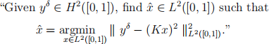
Since we consider the square of the kernel operator, the data for this question will be the square of the noisy yδ generated in Q2.(a). Abusively, these new squared data will be denoted by yδ in the remaining of this question.

(a) Give the Jacobian matrix involved in the local normal equations.

(b) Write the Gauss-Newton algorithm that solves the nonlinear inverse problem with a tol-erance of ε = 2.10−3 and a maximum number of iterations equal to 1000: use Tikhonov regularisation with parameter α = 10−3 to regularise the local normal equations in the Newton step. The algorithm should look like:

while the tolerance and the maximum number of iterations are not reached

Solve the local regularised normal equations to get δx

Update ˆxk+1 with δx

Update also δy from y δ and ˆxk+1

Increment the number of iterations

end

Does the algorithm converge? If yes, how many iterations were required to reach the tolerance?

Note: Do not forget to initialise ˆxk, ˆxk+1 and number of iterations.

(c) Plot on a new graph the exact parameter x(t) together with the Gauss-Newton regu-larised solution obtained ˆx (t) in (b). Comment on the global shape of the regularised solution ˆx

(t) compared with x(t), and on the boundary values at t = 0 and t = 1.