STAT 371 S24 Assignment #1

Hello, dear friend, you can consult us at any time if you have any questions, add WeChat: daixieit

STAT 371 S24 Assignment #1

Submission deadline: 11:59 pm Fri. May 31

1)  The Capital Asset Pricing model (CAPM) is commonly used to describe the relationship between the expected return and risk of a security (e.g. stock) in a given market. All investors assume a certain systematic or market risk associated with the market return, rm, for which they expect to be compensated above the risk free rate of return, rf (e.g. the return on a 10 year government bond). The difference between the expected market return and the risk free return, E(rm ) − rf , is known as the market risk premium. By investing in a security, investors assume an additional risk and thus expect a higher return on their asset.

In the standard CAPM model, this risk-reward relationship for any given stock is described by

E(r) = rf + β(E(rm ) − rf )

Or equivalently,

E(r) − rf = β(E(rm ) − rf )

where E(r) is the expected rate of return of the stock.

This model states that the risk premium of the stock, given byE(r) − rf , is linearly related to the market risk premium E(rm ) − rf . The slope parameter, β, is known as the stock’s beta, and is a measure of the stock’s risk or volatility relative to that of the market as a whole. For example, a beta value of 1.1 indicates that the stock’svolatility is 110% that of the market, whereas a stock with a beta of 0.5 suggests the stock is less risky than the market as a whole, possessing only 50% of the market’s volatility. Investors routinely use beta values in their investment decisions, and will select stocks based in part on the consistency between a stock’s beta and the investor’s level of risk-aversion.

The beta value for a given stock can be estimated by fitting the simple linear regression model

rt − rft = α + β(rmt − rft ) + εt

which can be expressed in the form

yt = α+ βxt + εt t = 1, 2, ..., T

where yt = rt − rft is the rate of return of the stock in excess of the risk-free rate at time t,  and xt = rmt − rft is    the market rate of return in excess of the risk-free rate at time t. Note that α can be loosely interpreted as the performance of a stock relative to that of the benchmark index.

For this assignment we will fit a simple linear regression  (SLR) model to monthly return rates over the past five years ( t = 1, 2,...,60) to estimate the beta of the Bank of Montreal (BMO) stock in the financial services sector. We will use the S&P/TSX composite index (TSXC) as a proxy for the market as a whole, and the yield on a 10-year Canadian government bond (GVTB) as a proxy for the risk-free rate of return.

To begin, download the capm_S24 csv file that contains monthly closing prices for BMO and TSXC, as well the annualized monthly rate of return for the government bond for the 5-year period from May 2019 to April 2024.

Before (or after) importing the dataset into R, you will need to transform the stock and index prices to monthly rates of return, where the rate of return of a stock for month t can be expressed as

As well, the given government bond annualized return rates, rat , will need to be converted to the monthly risk free rates:

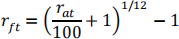
Note that by converting the prices to rates, the BMO and TSXC data will be reduced to 59 observations.

You will therefore need to remove the first observation (May 2019) from the government bond series before you calculate xt and yt .

a)  Before we fit the SLR model, yt = α+ βxt + εt , create a scatterplot of {xt,yt } . Does a linear model seem appropriate? What other characteristics of the plot do you see?

b)  Calculate the correlation coefficient, r, between xt and yt using R (a quick search will provide you with the appropriate function, if necessary).

c)  Use R to verify this value by calculating r directly from the definition provided in the lessons.

d)  Fit the SLR model

yt = α + βxt + εt εt ~ N(0,σ2 ) ind. t = 1, 2,...,59

to the data. Be sure to include the summary output in your assignment. See R output used in the lessons for additional assistance with relevant R code.

e)   Compare your estimate of beta with that in the BMO profile (BMO.TO) atca.finance.yahoo.com/

f)   Is the BMO stock volatility different from the market volatility?

i)   Answer this question by calculating a 95% confidence interval for the relevant parameter  using the confint function in R

ii)  Verify this interval by calculating, using R, the confidence interval directly from the  expression provided in lessons (that is, use R to obtain the relevant t value and to make the necessary calculations)

g)  According to the standard CAPM, alpha should be zero. Is the result of your regression analysis consistent with an alpha = 0? Answer this question by carrying out an appropriate hypothesis test (no calculations are required – just refer to the appropriate values in the output).

h)  Confirm the following output values by calculating these values in R directly from the definitions provided in lessons (be sure to show your R output for these calculations):

Relevant R functions:

> residuals(name.lm) #gives you the fitted residuals, ei , of the fitted model, name.lm.

> fitted(name.lm) #gives you the fitted values, , of the fitted model.

> sum(x^2)#gives you the sum of the squares of the data vector, x.

> pt(t, df) #gives you P(tdf < t)  , where tdf is at random variable with degrees of freedom, df .

i) α(^) ii) β(^) iii) se(β(^))         iv) σ(^) v) the p-value associated with H0  : β = 0

2)  Simulation is a useful method for understanding regression concepts and investigating properties of parameter

estimators. We will use R to generate random values of the response variable, Y, for the regression model Yi = β0  + β1xi1  + β2 xi 2  + β3 xi3  + β4 xi 4  + 8i 8i ~ N(0,σ2 ),ind.

based on a subset of the explanatory variates associated with the audit dataset. These explanatory variates can be found in the A1_variates dataset.

.     We will use parameter values -250000 (intercept), 50 (size),  -200 (age),  12000 (employees),  200000 (col), and 15000 for β0, β1, β2, β3, β4   and σ , respectively, to generate random values of Y associated with the given

set of values of your explanatory variates for this model. Include these values in your output. (Note that these somewhat arbitrary values for the (unknown) parameters are consistent with the fitted model of overhead vs. these variates)

Some R functions you may find useful:

•   rnorm(n,mu,sigma) #generates n random values from N(mu,sigma)

•   c(-250000, 50, -200, 12000, 200000) #creates the Beta vector

•   as.matrix(cbind(rep(1,n),A1_variates)) #creates X  matrix (i.e binds a column of ones to the matrix of explanatory variates)

•   A%*%B #yields the matrix product  (i.e., the inner product) of matrices A, B.

a) Using your student ID# as the seed *, generate (pseudo) random values of the response, overhead, for the given parameter values and set of explanatory variates.

*This can be accomplished with the command >set.seed(your ID#). This will not only ensure that each of you will generate a different set of values, but will also allow you to reproduce the results of your simulation if necessary.

Give your generated values so that the markers can verify that these values were generated from yourID number.

b)  Fit the linear model described above to the dataset containing the response variate and explanatory variates you generated.

•   A1sim.lm = lm(y~x1+x2+x3+x4) #fits a linear model to the data, where x1, . ..,x4 correspond to the explanatory variates.

•   summary(A1sim.lm) #displays a summary of the fit

c)   Confirm the parameter estimators  given  in the output by using R to calculate  β(^) = (XTX)−1XTy . As

always, be sure to include your R code.

d)  Based on your fitted model, provide a 95% confidence interval for β1 . Is this interval consistent with the value of β1  used to generate the response values?