Macroeconometrics Module 1: Graded Homework Problems

Hello, dear friend, you can consult us at any time if you have any questions, add WeChat: daixieit

Macroeconometrics

Module 1: Graded Homework Problems

Note: this problem set requires you to solve problems ''by hand'' and also to submit a Stata .do file. Handwritten solutions are perfectly fine as long as they are clearly legible. Your solutions to the analytical problems (that is, those to be solved by hand) should all be in a single .pdf file (if you do solve the problems by hand, then you can take pictures and convert to .pdf). Please put this .pdf file along with the Stata .do file in a .zip folder and upload this .zip file for your submission. VERY IMPORTANT: .pdf and .zip are the only formats accepted: solutions not submitted in .pdf and/or submitted in more than one file and/or submitted using any compression other than .zip are subject to being subtracted points or simply earning a grade of zero.

1. For a first order di§erence equation

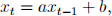
given the initial value x0 the solution is

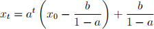
if a ≠ 1 and

if a = 1. Explain how the solution behaves in each of the following cases and draw a graph with an example.

(a) 0 < a < 1, x0 > x =  > 0. So, x0 is greater than the steady state value x, which is strictly positive.

(b) —1 < a < 0, x0 < x =  > 0. So, x0 is less than the steady state value x, which is strictly positive.

(c) a = 1, b > 0, x0 > 0:

(d) a = 1, b < 0, x0 > 0:

(e) a = 1, b = 0, x0 > 0:

2. Consider the following lagged income determination model:

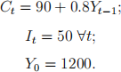
In equilibrium, Yt = Ct + It .

(a) Find the time path of national income Yt .

(b) Derive the steady state value of Y .

(c) Characterize the stability of the time path obtained in part (a).

3. (Note: the main references for this problems are the following two videos: ''M01.20: Stata: HP filter'' and ''M01.21: Stata: making a date.'') The Stata dataset realGDP.dta contains the variable rGDP, which is US real GDP (seasonally adjusted, at an annual rate) at quarterly frequency starting in the first quarter of 1947. Set up a Stata .do file called rGDP_control that does the following (in your code use commented lines of code to clearly indicate which part of the problem you are solving at each point):

(a) Clears the memory, loads the data, generates a date variable called quarter that starts in the first quarter of 1947 and formats the date variable so that it is ''readable by humans'' in line with the material covered in class and then uses tsset to set this variable up as the relevant time variable.

(b) Generates a variable called logGDP that is equal to the natural logarithm of rGDP (in Stata, to generate a variable called x that is equal to the natural log of y, run: gen x = log(y)).

(c) Generates a variable called C1600 that is equal to the cyclical component of logGDP using a smoothing parameter equal to 1600.

(d) Generates a variable called C10_5 that is equal to the cyclical component of logGDP using a smoothing parameter equal to 105.

(e) Uses the tsline command to plot C1600, names the graph "graph1," uses the replace command for the graph name and the nodraw option. Uses the tsline command to plot C10_5, names the graph "graph2," uses the replace command for the graph name and the nodraw option. Uses the graph combine command to put graph1 and graph2 on a same graph called ìgraph3îand uses the replace command for the graph name.

(f) Uses the sum command to obtain summary statistics for the variables C1600 and C10_5.

(g) Addresses the following question within the .do Öle itself by writing down the answer using comments: using your answers to part (e) and (f), which variable, C1600 or C10_5 is more volatilie and what explains this?