One, three... and five factors Lab Course 2

Hello, dear friend, you can consult us at any time if you have any questions, add WeChat: daixieit

One, three... and five factors

Lab Course 2 (DUE: Jun 2)

Group work: number of group members ≤ 3

Use a PPT (with names, student numbers of group members) to show your answers, send to CANVAS system.

1 FF Asset Pricing Model

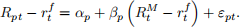
1.1 1 factor model

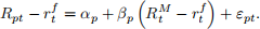
where

• Rp − rf: the excess return of a portfolio.

• RM −rf: the excess return on the market, is the value-weight return on all NYSE, AMEX, and NASDAQ stocks (from CRSP) minus the one-month Treasury bill rate (from Ibbotson Associates).

• βp: the sensitivity of the portfolio’s excess return to the market’s excess return (systematic risk)

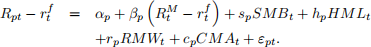
1.2 3 factor model

Fama and French (1993) advocate a three factor model to price portfolios. That is, a portfolio’s excess return Rt could be explained by three factors.

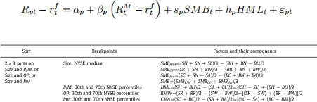
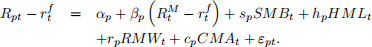
Figure 1: Construction of Factors

1.3 5 factor model

Fama and French (2015) update the model with a five factor model.

2 Data (196307-201502)

You could get two txt files

(1) F-F_Research_Data_5_Factors_2x3.txt : Fama/French 5 Factors

(2) 25_Portfolios_5x5: 25 Portfolios Formed on Size and Book-to-Market

(3) copy data in txt to excel, match the two part

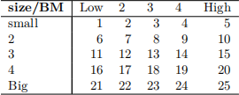
This file was created by CMPT_ME_BEME_RETS using the 201502 CRSP database. It contains value- and equal-weighted returns for the intersections of 5 ME portfolios and 5 BE/ME portfolios. The 25 portfolios are listed as below.

3 Program

Use stata do file to do the following work.

1. Summarize the basic statistics (mean, std,...) for these variable. Is  stationary and weakly dependent? (Hint: check corr)

2. Run 25 simple regression

test H0 : αp = 0, and collect 

3. Run 25 3-factor regression

4. Run 25 5-factor regression

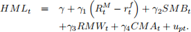
We could show that HML is redundant. That is, test whether H0 : γ = 0 holds for

5. Choose one of the 25 regressions in (3)

(a) Test whether conditional heteroskedasticity exists.

(b) Test whether conditional serial correlation exists.

6. EMH1. Test efficient market hypothesis

Run the AR(p) model (use AIC to determine p)

test H0 : ρ1 = ... = ρp = 0.

What’s your conclusion about market efficiency?

7. EMH2. Test whether January Effect exists.

Rpt = α0 + α1Jant + ut

(a) Give some reasons for the existence of Juanuary effect.

(b) Split the data into two groups: before Dec 1985 and after. Test January effect for each group. Why are the results different?

(c) Is there Feburary Effect? or others? How to test?

(d) If we propose January effect is associated with firm’s size, how to test it?

(e) If we propose January effect is associated with β in CAPM, how to test it?

8. Present and summarize what you find through the results. (refer to Fama French (2015), table 7)

4 Report

Use a PPT to present your results and how you interpret these results.

5 Stata skills

• Time series in STATA: time variable and plot

tsset tm, month

tsline rf

• How to collect 25 regression results automatically?

– Method 1. for loop

display "asset" _col(10) "coef" _col(30) "std" _col(50) "t"

forvalues i=1(1)25{

quietly regress p`i' mktrf

* display : num of regression; beta coefl; beta std; beta t

display `i' _col(10) _b[mktrf] _col(30) _se[mktrf] _col(50) _b[mktrf]/_se[mktrf]

}

– Method 2. postfile

use ff5data.dta, clear

tempname table

postfile `table' b1 se1 df using "ffres.dta", replace

forvalues i=1(1)25{

quietly regress p`i' mktrf

post `table' (_b[mktrf]) (_se[mktrf]) (e(df_r))

}

postclose `table'

use ffres, clear

generate t1 = b1/se1

*generate p1 = (1-normal( abs(tx1)) )*2

generate p1 = ttail( df,abs(t1)) *2

list

• Extension*: time variables

* date function: from string variable (month_str) to stata dates (tm2)

gen td = date(month_str, "YM")

format gen tm2 = mofd(td)

* declare data to be time series

tsset tm2, month

* gen calendar month

gen month_cal = month(td)

6 Useful links

1. Basic introduction

http://en.wikipedia.org/wiki/Fama%E2%80%93French_three-factor_model

2. Updated data

http://mba.tuck.dartmouth.edu/pages/faculty/ken.french/data_library.html

3. Readings

Fama E F, French K R. Common risk factors in the returns on stocks and bonds[J]. Journal of Financial Economics, 1993, 33(1): 3-56. (google scholar citation: 22267)

Fama E F, French K R. A five-factor asset pricing model[J]. Journal of Financial Economics, 2015, 116: 1-22.

Thaler R H. Anomalies: the January effect. Journal of Economic Per-spectives. 1987, 1(1):197-201.