Systems Modelling and Analysis – Assignment 3

Hello, dear friend, you can consult us at any time if you have any questions, add WeChat: daixieit

Systems Modelling and Analysis – Assignment 3

Due: Friday 24/05/2024 by 11:59:00 pm. To be submitted individually using the online multiple choice/fill-in-the-blank system on Canvas.

Input Format:

Do not add + in front of positive numbers, e.g. 0.1 should be used not +0.1. If the answer is negative then use − in front, e.g., −0.1 is fine.

Add a zero before decimals, e.g., 0.1 should be used not .1

Do not use scientific notation, e.g., 12400 should be used not 1.24e4.

Do not add units, e.g., 0.1 should be used not 0.1m.

If you do not follow these input format the answers will be marked wrong.

Assignment Background

This assignment is a continuation of Assignment 1 and 2, where you have modelled the DC-motor driven positioning system. No material from Assignment 1 or 2 is required to complete this assignment.

Recall that V (s) = L {v(t)} is the voltage supplied to the DC motor and Y (s) = L {y(t)} is the dartboard’s vertical position. The transfer function  is exactly

Please run the code in MATLAB:

num = [40714 508929 440935714];

den = [1 67.54 137398 2227095 1054370920 1388909637 5830019524 -0.0079];

G_OL = tf(num,den);

Assume zero initial conditions when required.

Part 1: Dartboard Positioning System, Sinusoidal Inputs

Q1-2. Using MATLAB, plot the Bode diagram of GOL(s) (with a grid). Observe the behaviour at low frequencies and at high frequencies (for both magnitude and phase).

(Q1) Is the gain larger at low or high frequencies? [Canvas Input: Select Low or High]

(Q2) Is the phase lag smaller at low or high frequencies? [Canvas Input: Select Low or High]

Q3-4. Apply sinusoids of varying amplitude (v = Asin(t)) and observe the steady-state behaviour of y(t)

(i.e. yss(t)). For each question below, you are given a specific value A. Use this value of A to answer the question.

(Q3) What is the phase shift between yss(t) and v(t)? (The answer should be in degrees and in the range [−180o , 180o ))?

(Q4) What is the average value of yss(t)?

[Canvas Input: Two signed numbers - 5% tolerance allowed]

Q5-6. Now apply sinusoids of varying frequency (v = 1000 sin(ωt)) and observe the steady state behaviour of y(t) (i.e. yss(t)). For each question below, you are given a specific value ω, use this value of ω to answer the question.

(Q5) What is the phase shift between yss(t) and v(t)? (The answer should be in degrees and in the range [−180o , 180o ))?

(Q6) For yss(t), what is the maximum deviation from its average value?

[Canvas Input: Two signed numbers - 5% tolerance allowed]

Q7. Amplify the voltage supplied to the motor by a constant A, so that v(t) = A sin(t) is supplied to the motor.

Find the largest integer A such that |y(t)| ≤ 0.5[m]. [Canvas Input: One integer]

Hint: It is sufficient to use a trial-and-error approach.

Part 2: Dartboard Positioning System, Closed-Loop Control and Discrete Systems

To simplify the problem now approximate the open-loop system with a lower order system as follows: 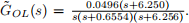 Use this for all subsequent analysis involving the open-loop system. Part 1 has shown us that tuning parameters A and w for input v = Asin(wt) to achieve a desired behaviour of y(t) is not efficient, so we turn again to closed-loop control. A position sensor is purchased to measure y(t) accurately. First, use a controller C(s) = K such that the voltage supplied to the motor is v = K(r − y), where r is a reference signal.

Q8-13. Produce the Bode Diagram for the closed-loop system with K = 100. On the Canvas quiz, you will be given different values of ω.

(Q8-10) Find the values of gain [dB] for the given values of ω. [Canvas Input: two signed numbers - 5% tolerance allowed]

(Q11-13) Find the values of phase [deg] for the given values of ω. (The answer should be in degrees and in the range [−180o , 180o )) [Canvas Input: two signed numbers - 5% tolerance allowed]

Q14-16. For K = 5000, plot r(t) = 10 sin (ωt) and the corresponding y(t) for ω = 0.73 [rad/sec], ω = 7.3 [rad/sec], ω = 73.0 [rad/sec] (two graphs on the same axes for each frequency). Capture enough time to show the steady-state response of y(t).

Find the value of y(t) − r(t) when t is 50 s for ω = 0.73, 7.3, 73.0 [rad/sec]. [Canvas Input: Three signed numbers - 5% tolerance allowed]

For K = 88 and the reference signal r(t) = 0.1 sin(t), we will find the magnitude and the phase-shift of yss(t) in three ways:

Q17-18. Graphically, by reading values from the Bode diagram of the closed-loop system. Using the Bode diagram, find the magnitude [dB] and phase [deg] of yss(t). (The answer of the phase should be in degrees and in the range [−180o , 180o ))[LMS Input: Two signed numbers - 5% tolerance allowed]

Q19-20. Graphically, by reading values from the response plot y(t) after it reaches a steady-state. For the response plot y(t), let the first peak in y(t) after t = 50 sec be at time ty. Let t1 be the closest r(t) peak preceding time ty and t2 be the closest r(t) peak following ty.

(Q19) What is y(ty)? [Canvas Input: One signed numbers - 5% tolerance allowed]

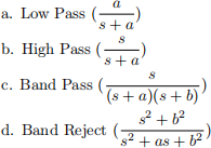
(Q20) Select the equation that approximates the phase [deg] of yss(t) from Figure 1. [Canvas Input: One integer]

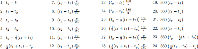
Figure 1: Selection options for Q19

Q21-22. Analytically, by substituting s = j · 1 into the transfer function of the closed-loop system. Find the (Q21) real and (Q22) imaginary parts of the resulting complex number. [Canvas Input: Two signed numbers - 5% tolerance allowed]

Q23-24. We wish to avoid the dartboard going outside the boundary at a steady-state mode (if there is a finite number of exits - it is acceptable). Assume that we would like to operate at high frequencies (i.e. ω > 1 rad/s). If K = 3000 and the total width of the safe zone is 1500 [mm], which frequencies ω should not be used where the reference signal is r(t) = 0.5 sin (ωt)[m]?

Using the Bode diagram, find the range ω ∈ [ωmin, ωmax] [rad/sec] such that the reference signal is not suitable. [Canvas Input: Two signed numbers - 5% tolerance allowed]

Set K = 800 from now on forming a closed loop system GCL(j, ω). We would like to address the long phase-lag produced in this system when r(t) = 0.1sin(t).To improve performance, we will use an additional controller with transfer function 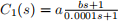 outside the feedback loop such that

(R(s) is the Laplace transform of r(t)). We would like the output y(t) to exactly match the reference signal r(t) = 0.1sin(t) and can do so by tuning the values of a and b in the controller.

Q25-26. Find |GCL(jω)| [unitless] and ∠GCL(jω) [deg] for ω = 1 rad/sec for the original closed loop system GCL(jω). (The answer of the phase should be in degrees and in the range [−180o , 180o )) [Canvas Input: Two signed numbers - 5% tolerance allowed]

Q27-28. Find a and b such that the output for the new system matches the reference signal (yss(t) = r(t) = 0.1 sin(t)). [Canvas Input: Two signed numbers - 5% tolerance allowed]

Q29-32. Reflect on the usage of closed-loop control for the positioning system. What are the benefits which can be achieved by using it, compared to open-loop control?

Select true or false for the following statements

The closed loop control system:

(Q29) does not require a sensor. [Canvas Input: Select True or False]

(Q30) can allow the poles of the system to be moved to the LHP and make the system exponentially stable. [Canvas Input: Select True or False]

(Q31) can allow better tracking of a reference signal. [Canvas Input: Select True or False]

(Q32) results in a system that is more robust to errors due to the presence of feedback. [Canvas Input: Select True or False]

After analysing the system in continuous time, now investigate how the system behaves in discrete time.

Q33. Start by converting the continuous-time system ˜GOL(s) into a discrete-time system ˜GOL(z) using the bilinear transformation (Tustin’s Method) with the sampling time T = 1s. Let the open-loop transfer function be  What is the value of b4? [Canvas Input: one signed numbers - 5% tolerance allowed]

Q34. Then calculate the discrete-time frequency wd [rad/s] corresponding to the continuous-time operating frequency wa = 1 [rad/s]. What is the value of wd? [Canvas Input: one signed numbers - 5% tolerance allowed]

Q35-37. Lastly, apply a known input, collect data from the sensor and use that data to perform a system ID to validate the model of the system you have worked with.

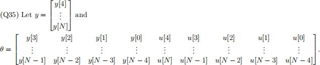
Which of the options in Figure 2 is the correct parameter vector p? [Canvas Input: one integer]

(Q36-37) Let the input u[k] = {0, 0.2, 0.35, 0.68, 0.83, 0, 0, 0, . . . } (i.e. u[0] = 0, u[1] = 0.2, u[2] = 0.35, u[3] = 0.68, u[4] = 0.83 and u[i] = 0 for i > 4). The output data collected by the sensor is given in y_dat.mat.

Perform a system ID on the given data set. Let the open-loop transfer function obtained from the data be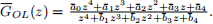 

Q36. What is the maximum deviation in the parameter on the numerator 

Q37. What is the maximum deviation in the parameter on the denominator

 [Canvas Input: Two signed numbers - 5% tolerance allowed]

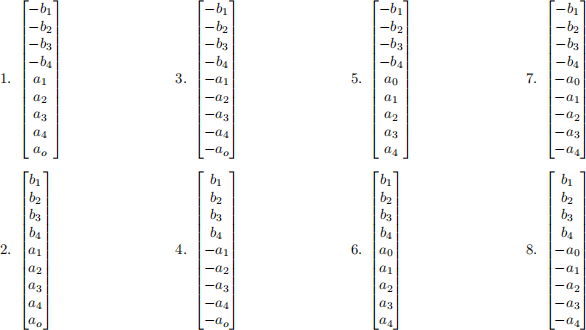
Figure 2: Selection Options for Q35

Part 3: Filtering Signals

You will now be investigating the effect of different transfer functions on multi-tone audio files by analysing the frequency content of the signals and the frequency response of the transfer functions.

Note that in all of Part 3 you may ignore the influence of the transient response. That is, you only need consider the steady-state response given by the frequency response G(jω).

Q38. The magnitude of the Discrete Fourier Transform of two signals are given in Figure 2. Signal 2 is Signal 1 after being passed through some transfer function. Based on the figures, what type of transfer function was used? [Canvas Input: Multiple Choice]

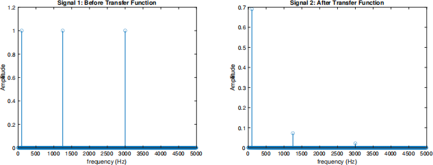
Figure 3: Signal Before and After Passing Through Transfer Function

In the Canvas quiz introduction, you are given 10 audio files (.wav). Each audio file is a selection of multiple pure tones, 5 seconds long. Download the audio files. Use the function audioread() to load these audio files into your MATLAB workspace.

Example (’tones1.wav’):

>‌> [signal1, Fs1] = audioread(’tones1.wav’);

signal1 will be a vector of numbers representing the audio signal ’tones.wav’. Fs1 will be the sampling frequency, in Hz.

The magnitude of the Discrete Fourier Transform for ’tones1.wav’ is given in Figure 3, for your reference.

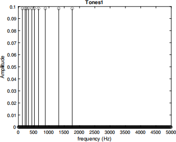
Figure 4: Frequency Content of tones1.wav

Q39-40. Load ’tones3.wav’ and, using MATLAB, determine the frequency content of the signal. What are the two frequencies (Hz) present in the signal with the largest magnitudes? [Canvas Input: Two signed numbers - 5% tolerance allowed]

’tones[1-5].wav’ are 5 different multi-tone recorded audio signals. These signals are used as the inputs to some transfer functions and recorded again to produce 5 new audio signals: ’output[a-e].wav’. Some noise is introduced into the audio signals during the recording process.

Q41. Match the original audio files (’tones[1-5].wav’) to the corresponding output audio files (’output[a-e].wav’). [Canvas Input: Matching]

You are also given a data matrix ’tf_data.mat’. Load the file into your MATLAB workspace (>‌> load(’tf_data.mat’)). This matrix represents the frequency response, G(jω), of 16 different transfer functons. Each original audio file was used as the input to one of these transfer functions to produce the output files. We will now identify which transfer functions were used.

The matrix is 16x25001, each row (1-16) representing a different transfer function. The following 16 Figures are the Bode Diagrams for each transfer function in the same order as is presented in the matrix, for your reference.

The matrix gives 25001 complex values for each transfer function. Each complex value is the transfer function evaluated at a different frequency. These frequencies (in Hz) are given in ’freq.mat’.

Hint: You may find the MATLAB command frd() useful to load the data into a frequency response data model. In this way you can more easily plot the Bode plots using the bode() command. For example:

>‌> G = frd(resp,omega);

>‌> bode(G);

Be careful with units, omega should be in rad/s.

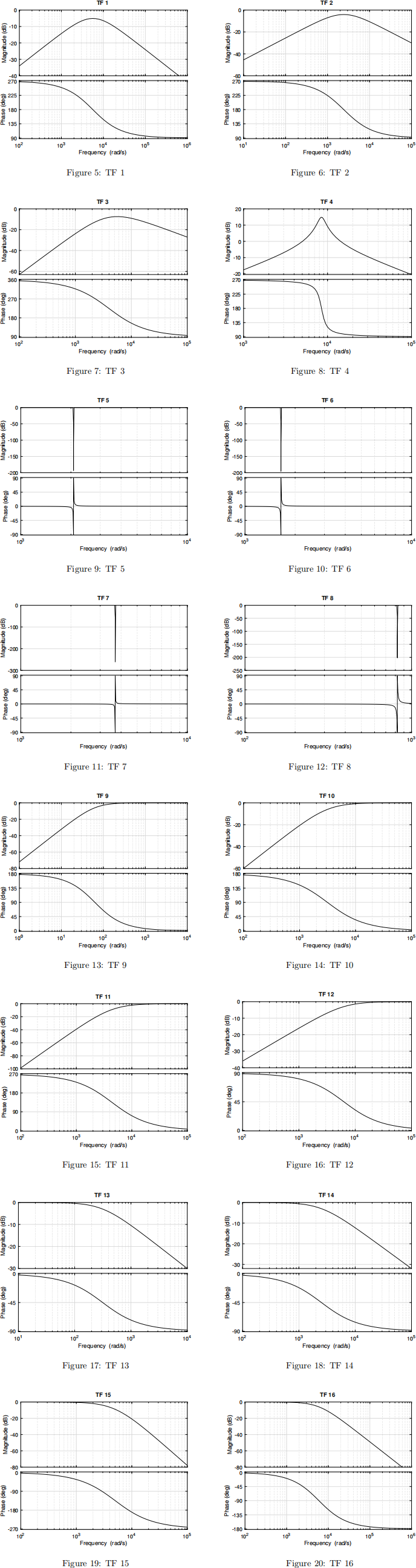
Q42. Use these complex values to determine the effect the transfer functions will have on the frequen-cies present in the original signals. Match the original audio files to the corresponding transfer functions. [Canvas Input: Matching]

Note: ’TF 1’ is the transfer function described by the first row of the data matrix and the first Bode plot given. TF 2-16 follow in the same fashion.