关键词 > MA2034
MA 2034 Worksheet 4 Spring 2024
发布时间:2024-05-20
Hello, dear friend, you can consult us at any time if you have any questions, add WeChat: daixieit
MA 2034
Worksheet 4
Spring 2024
Predator-Prey Modeling
The traditional Lotka-Volterra predator-prey model is a fundamental ecological concept used to describe the interactions between two species in an ecosystem, typically a predator and its prey. Developed independently by Alfred Lotka and Vito Volterra in the early 20th century, this model provides insights into how the populations of predator and prey species can change over time in response to each other’s presence. The Lotka-Volterra model has been applied to competition among pathogens, economic situations and competition in the corporate worlds, as well as social media.
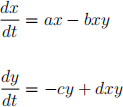
The Lotka-Volterra model consists of two coupled nonlinear first-order differential equations that describe the dynamics of the predator and prey populations. These equations are as follows:

dx/dt represents the rate of change in the prey population x over time, and dy/dt represents the rate of change in the predator population y over time. and a,b,c,d are positive constants where:
. a represents the intrinsic growth rate of the prey population in the absence of predators.
. b represents the rate at which predators y consume or kill prey individuals.
. c represents the predator’s death rate when there is no prey to consume.
. d represents the rate at which predators reproduce as a result of consuming prey.
An entertaining and effective introduction to the Lotka-Volterra Predator-Prey system can be found in this video Predator Prey Numberphile
1. PART I: Investigating Key Concepts Using Graphs.
Although the Lotka-Volterra system can be solved analytically, the solutions are beyond the scope of our class, so we will will explore key concepts such as Cyclic Behavior, Parameter Sensitivity and Equilibrium Points and other features of the Lotka-Volterra predator-prey model graphically by using the Slopes App by Tim Lucas.
You can use any other app or program to graph the solutions of the predator-prey system, but the Slopes App is really convenient.
Cyclic Behavior: The model predicts that predator and prey populations can exhibit cyclic or oscillatory behavior over time. When the prey population is high, it provides abundant food for predators, causing the predator population to increase. As the predator population increases, it exerts greater predation pressure on the prey, causing the prey population to decline. This, in turn, leads to a decrease in the predator population due to reduced food availability. The cycle then repeats.
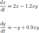
Parameter Sensitivity: The behavior of the model is highly sensitive to changes in the values of its parameters, such as the intrinsic growth rates, predation rates, and death rates. Small changes in these parameters can lead to significant differences in the dynamics of the predator-prey system. To investigate how the solutions depend on the parameters we will use this system:
For each of the constants a,b,c,d, you are to individually look at what the effect of changing that constant has on the amplitude and period of the solutions. Use the Slopes App to investigate the effect changing the parameters on the solutions curves. Upload your answers as a pdf file to GS.
For the following questions (except questions 11 and 12), keep the initial conditions at x(0) = 1, y(0) = 1.
1. If a = 2 is doubled to a = 4, what is the effect on the amplitude and period of both x(t) and y(t)? What does a represent in the Lotka-Volterra Models? Does the effect on the solutions curves make sense?
2. If a = 2 is halved to a = 1, what is the effect on the amplitude and period of both x(t) and y(t)? Does the effect on the solutions curves make sense?
3. If b = 1.2 is doubled to b = 2.4, what is the effect on the amplitude and period of both x(t) and y(t)? What does b represent in the Lotka-Volterra Models? Does the effect on the solutions curves make sense?
4. If b = 1.2 is halved to b = 0.6, what is the effect on the amplitude and period of both x(t) and y(t)? Does the effect on the solutions curves make sense?
5. If c = 1 is doubled to c = 2, what is the effect on the amplitude and period of both x(t) and y(t)? What does c represent in the Lotka-Volterra Models? Does the effect on the solutions curves make sense?
6. If c = is halved to c = 0.5, what is the effect on the amplitude and period of both x(t) and y(t)? Does the effect on the solutions curves make sense?
7. If d = 0.9 is doubled tod = 1.8, what is the effect on the amplitude and period of both x(t) and y(t)? What does d represent in the Lotka-Volterra Models? Does the effect on the solutions curves make sense?
8. If d = 0.9 is halved to d = 0.45, what is the effect on the amplitude and period of both x(t) and y(t)? Does the effect on the solutions curves make sense?
9. What is the effect on the solution curves of setting b = 0?
10. What is the effect on the solution curves of setting d = 0?
11. What effect does changing the initial values have on the solution curves?
12. Upload a graph for the case when all of the default values in slopes app are doubled and the initial value is x(0) = 5, y(0) = 2 and describe how the graphs differ from the graph of the default values.
Equilibrium Points: The model has equilibrium points where both populations remain constant over time. These equilibrium points can be stable or unstable, depending on the values of the model parameters. A stable equilibrium represents a situation where predator and prey popula- tions coexist in a relatively stable manner. In the Lotka-Volterra Model it is rare to find perfect equilibrium solutions, more often the solutions exhibit oscillatory behaviour around the equilibrium points rather than staying at them.
To find the equilibrium points for this system we set both dx/dt and dy/dt to zero and solve
We find we have 2 sets of equilibrium values, (0, 0) when both predator and prey populations vanish, and (c/d,a/b) when there are just enough prey to support a constant predator population but there are not too many predators.
Answer the following question for the system shown below.
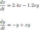
11. Find the equilibrium values for the system and use the Slopes App Phase Plane Activityto graph a solution in the plase plane with intial conditions as close as you can get to the equilibrium value. Upload your file to GS showing both the solution and the phase plane portrait.
2. Part II Real World Examples.
Pesticides Pesticides that kill all insect species are not only bad for the environment, they can also be inefficient at controlling the pest species and can have unintended consequences. Suppose a pest insect species in a particular field has a population x(t) at a particular time t, and suppose its primary predator is another insect species with population y(t) at time t. Suppose the population of these species are accurately modeled by the system
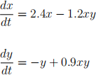
Also suppose that at time t = 0 a pesticide is applied to the field that reduces both the pest and predator populations to a very small but non-zero numbers.
1. Use the Slopes app (or other similar app) to investigate what happens to this system. Choose 2 sets of initial conditions, both near zero. Let x(0) = 5y(0). Whatever initial values you choose for your first set, the second set of values should be 1/100 of the first. Plot the solutions. Be sure to expand the scale if necessary, and look out to times ’far’ in the future. You will upload these solution curves to GS. You should also try other scenarios to get a feel for what can happen, but you only need to upload 2 graphs.
2. If the pest could be eliminated, would it be eliminated for all time? Explain your answer. Do you think that it is realistic to completely eliminate the pest?
3. If the pest could be eliminated, would it’s predator be eliminated for all time too? Explain your answer.
4. Is the behavior of the pest that you found advantageous for the farmers? For the producers of the pesticides?
5. Write a short paragraph or two ’Letter to the Editor’ to a Newspaper (or blog) warning about the implications and possible unintended consequences that pesticide applications can have on pest populations.
Reintroduction of Wolves into Yellowstone National Park, Wyoming.
The reintroduction of wolves to Yellowstone National Park is a fascinating case study in ecosys- tem management and conservation biology. Here’s a brief overview of key aspects of this case: In 1995, wolves were reintroduced to Yellowstone National Park after being eliminated in the 1920s. The primary goal was to restore a vital part of the park’s ecosystem that had been missing for nearly 70 years.
The initial reintroduction involved 31 wolves from Canada. These wolves were released in sev- eral groups, and their populations grew steadily, benefiting from the abundant prey and lack of human interference. The reintroduction of wolves had profound effects on the Yellowstone ecosystem which are nicely summarized in this interesting (and somewhat controversial) video How Wolves Change Rivers
While the Lotka-Volterra model simplifies complex ecological interactions, it provides a useful framework for understanding predator-prey relationships in nature. It’s important to note that ecological data can be complex and context-dependent. The interaction between wolves and elk in Yellowstone is influenced by many factors beyond just simple population counts, including environmental changes, human activities, and the presence of other predators and prey species and many modified models have been applied to this case.
Expanding the Model
One modification of the predator-prey model would be to assume that, in the absence of predators, the prey population obeys a logistic rather than an exponential growth model. One such model is provided by the system of differential equations given by
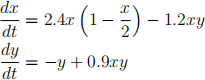
6. Find the equilibrium points for the system shown above. Explain the significance of these points in terms of the predator and prey populations.
7. How would you modify the above equations to include the effect of hunting on the prey at a constant rate of α units per unit of time (matching the units in the above equation, whatever they are chosen to be). In the case of elk and wolf example, the elk are hunted in addition to being prey for the wolves.
8. How would you modify the above equations to include the effect of hunting on the predators at a rate proportional to the number of predators?
9. Suppose the predators discover a second, unlimited food source but they still prefer to eat prey when they can catch them. How would you modify the above equations to include this assumption.
