关键词 > STATS3860B/9155B

STATS 3860B/9155B Assignment 4 Winter 2024

发布时间：2024-05-20

Hello, dear friend, you can consult us at any time if you have any questions, add WeChat: daixieit

Assignment 4

STATS 3860B/9155B

Winter 2024

Question 1

a) In a small pilot study, researchers compared two groups of 4 turbine wheels under low humidity and two groups of 4 turbine wheels under high humidity conditions. The goal is to investigate if humidity is related to the development of ﬁssures. If Y = number of turbine wheels that develop ﬁssures, then assume that Y ∼ Binomial(n = 4, p = pL ) under low humidity, and Y ∼ Binomial(n = 4, p = pH ) under high humidity. Write out the log-likelihood function log L(pL , pH ) using the observed data in Table 1 and simplifying where possible. Show all the details.

b) Using the log-likelihood function obtained in part a), calculate the maximum likelihood estimates (MLEs) of pL and pH , L and H . Show all the details.

Table 1: Pilot study data.

Turbine group	1	2	3	4
Humidity	Low	Low	High	High
n = number of turbine wheels	4	4	4	4
y = number of turbine wheels with ﬁssures	1	3	1	0

c) We ﬁt the following Binomial regression model to the data in Table 1 and present the estimated coeﬃcients below. Show how the Binomial regression estimated coeﬃcients are related to the MLEs, L and H , obtained in part b). Show all the details.

y = c(1,3,1,0)

Humidity = factor(c("Low","Low","High","High"),levels=c("Low","High"))

data_pilot <- data.frame(y, Humidity)

fit_pilot <- glm(cbind(y,4-y) ~ Humidity,data=data_pilot,family=binomial)

round(coef(fit_pilot),6)

## (Intercept) HumidityHigh

## 0.00000 -1.94591

Question 2

This question refers to exercise 4 of Chapter 8 of the textbook; however, instead of working with the Galapagos data and the Poisson model, you will now work with the dataset in Table from Question 1 and the Binomial model. The purpose of this question is to reproduce the details of the GLM ﬁtting of this data via the IRWLS algorithm.

a) Consider the Binomial regression model ﬁtted in part c) of the previous question. Report the estimated coeﬃcients and the deviance.

For parts b), c), d), e), f) and g), refer to Exercise 4, Chapter 8 of the textbook (page 172) and consider a Binomial GLM.

Question 3

The dataset Weekly contains 1089 weekly observations on the following variables regarding the S&P 500 stock market. Note: this question does not require any coding. As in the midterm exam, you should answer the parts below based solely on the information provided.

• Direction: a binary response with levels Down (0) and Up (1) indicating whether the market had a positive or negative return on a given week.

• Lag2: percentage return for 2 previous weeks.

• Volume: a factor with levels High (1) and Low (0) indicating if the volume of shares traded was high or low on a given week.

head(Weekly, 5)

## Lag2 Volume Direction

## 1 1.572 Low Down

## 2 0.816 Low Down

## 3 -0.270 Low Up

## 4 -2.576 Low Up

## 5 3.514 Low Up

summary(Weekly)

## Lag2 Volume Direction

## Min. :-18.1950 Low :544 Down:484

## 1st Qu.: -1.1540 High:545 Up :605

## Median : 0.2410

## Mean : 0.1511

## 3rd Qu.: 1.4090

## Max. : 12.0260

a) A logistic regression model was ﬁtted to the Weekly dataset. The resulting linear predictor estimates are plotted against Lag2 and shown in the ﬁgure below. Based on this plot, what is the logistic regression model ﬁtted to these data? What is the total number of model coeﬃcients? Write both the model equation (showing the link function and its relationship with the predictors) and the glm() code for it. Explain in details your rationale.

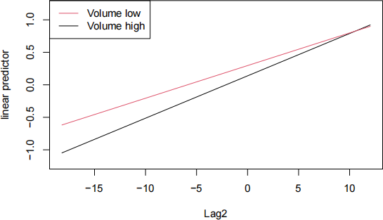
b) The intercept and slope of the black line in the plot shown in part a) are:

## (Intercept)

## 0.138

## Lag2

## 0.065

And the intercept and slope of the red line in the same plot are:

## (Intercept)

## 0.296

## Lag2

## 0.05

Interpret the slope of each line (black and red) in terms of odds of direction Up (positive market return).

c) What about the intercepts in part b)? Is there a practical interpretation for them? Explain.

d) Based on the slope and intercept values presented in part b), what are the estimated coeﬃcients for the model you described in part a)? Show all your work.

Question 4

Refer to Exercise 1 page 251 of the textbook. Dataset ratdrink. Work on parts a) to e).

library(faraway)

str(ratdrink)

## ' data. frame ' : 135 obs . of 4 variables:

## $ wt : num 57 86 114 139 172 60 93 123 146 177 . . .

## $ weeks : int 0 1 2 3 4 0 1 2 3 4 . . .

## $ subject: Factor w/ 27 levels "1","2","3","4",..: 1 1 1 1 1 2 2 2 2 2 . . .

## $ treat : Factor w/ 3 levels "control","thiouracil",..: 1 1 1 1 1 1 1 1 1 1 . . .

Question 5

Refer to Exercise 2 page 251 of the textbook. Dataset hprice. Work on parts a) to g).

library(faraway)

str(hprice)

## ' data. frame ' : 324 obs . of 8 variables:

## $ narsp : num 4.22 4.27 4.33 4.36 4.39 . . .

## $ ypc : int 13585 14296 15413 16490 17634 18210 17958 18659 19360 15354 . . . ## $ perypc : num 6.47 5.23 7.81 6.99 6.94 . . .

## $ regtest: int 20 20 20 20 20 20 20 20 20 18 . . .

## $ rcdum : Factor w/ 2 levels "0","1": 1 1 1 1 1 1 1 1 1 1 . . .

## $ ajwtr : Factor w/ 2 levels "0","1": 1 1 1 1 1 1 1 1 1 1 . . .

## $ msa : Factor w/ 36 levels "1","2","3","4",..: 1 1 1 1 1 1 1 1 1 2 . . . ## $ time : int 1 2 3 4 5 6 7 8 9 1 . . .

Question 6

The dataset teengamb in the library faraway concerns a study of teenage gambling in Britain. Take the variables gamble as the response and income as the predictor.

a) Plot the data and ﬁt a curve using kernel smoothing with a cross-validated choice of bandwidth. Plot the ﬁt on the top of the data. Does the ﬁt look linear?

b) Fit a curve using smoothing splines with the automatically chosen amount of smoothing (by cross-validation). Display the ﬁt on the data and report the eﬀective degrees of freedom.

c) Fit a curve using smoothing splines with somewhat larger degrees of freedom than in

part b). Compare the results with part b). Was the automatic choice satisfactory?