关键词 > PHYS3x34
PHYS3x34 Computational Physics 2024
发布时间:2024-05-17
Hello, dear friend, you can consult us at any time if you have any questions, add WeChat: daixieit
PHYS3x34 Computational Physics 2024
Instructions
Provide written answers including explanations, where required, for all questions. In each case where a question involves writing or modifying an existing MATLAB code, include a listing of the code as part of your assignment submission. You are reminded that your work on this assignment must be your own. For code, this means the new working parts of the code needed for a problem must be your own work.
The two-body problem
The second lecture and lab considered the central force (Kepler) problem, concerning the motion of a planet or comet, around a much more massive object, the Sun. In this problem, we relax the assumption that the Sun is ixed in space, seeking numerical solutions to the resulting general two-body problem, which describes the dynamics of two masses subject to their mutual gravitational attraction.

Question A: Setting up the problem
The equations of motion of two objects under gravity may be written in SI units as:
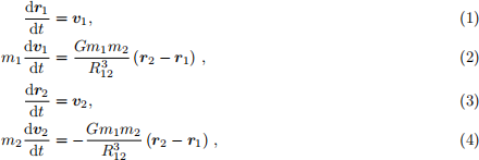
where r1 and r2 are the positions of the objects, v1 and v2 are the velocities, m1 and m2 are the values of the masses, R12 = jr2 - r1 j is the distance between the objects, and G 6.67 10- 11 kg- 1 m3 s-2 is the gravitational constant.
(i) [2 points] The centre-of-mass (COM) of the system is

Show that the center of mass has zero acceleration.
(ii) [2 points] By applying a transformation to the COM frame:

show the equations of motion may be written as:
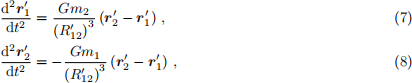
where 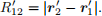
(iii) [3 points] By introducing the non-dimensional variables

for i = 1, 2 with the choice

show that Eqs (7) and (8) can be rewritten as:
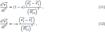
where a = m1 /M. Explain all steps in your working.
(iv) [2 points] The angular momentum of the system, in non-dimensional units with respect to the centre of mass (COM), is

Show that the angular momentum of the system is conserved during the motion. This result means
that the motion occurs in a plane, so we can assume 
(v) [2 points] The total energy of the system (in dimensional units in the COM frame) is

Show that Eq. (14) can be rewritten in non-dimensional form as
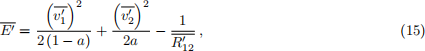
where 
Question B: Numerical solutions (13 points)
In this question we use the equations from Question A, but drop the primes and bars to simplify the notation. We will indicate when we are working in the centre-of-mass frame and in non-dimensional units.
(i) Numerical solution with Velocity–Verlet.
Consider the numerical solution of the non-dimensional form of the equations of motion in the centre of mass frame, Eqs (11), (12) using the Velocity–Verlet method. This method can be written

where i = 1, 2 identiies the object, n indicates the time according to tn = (n - 1)τ , and τ is the time step.
i. [2 points] Write code to calculate a numerical solution of the two-body problem using the Velocity– Verlet scheme. Use the initial conditions: r1 ; 1 = [1, 0] and v1 ; 1 = l0, 2-3/2]. Choose the initial value r2 ; 1 which puts the centre of mass at the origin. The initial condition v2 ; 1 is determined by v1 ; 1 and the mass ratio a, because Eqs (11) and (12) assume the velocity of the centre-of-mass of the system is zero. Provide your code.
ii. [2 points] Calculate a test solution for the case a = 0.5, with a time step τ = 0.05 for a total time T = 25/2π . For the given initial conditions, mass ratio, and total integration time, both masses should follow the unit circle and complete one orbit. (If you do not obtain this result, your code is not working correctly).
Have your code animate the solution in the same way as the code kepler_verlet.m (from the second lecture), showing at each time step the positions of the objects, and also the orbits over the preceding time steps.
Also have your code calculate the total energy of the system (in non-dimensional units in the centre of mass frame) at each time step using Eq. (15), and at the end of the integration, plot the total energy versus time. Include two igures with your solution: one showing the orbits and inal positions of the objects, and a second showing the total energy versus time.
iii. [2 points] Run your code for the case a = 1/3, with the same initial conditions on r1 ; 1 and v1 ; 1 and with the centre of mass at the origin. You may need to reduce your time step to obtain an accurate numerical integration with a = 1/3. Include the two same igures as in the previous part, showing the orbits and the variation of energy with time. Briely explain how you know the solutions are accurate, and describe the orbit obtained for the case a = 1/3.
(ii) Numerical solution with RK4 . Consider the numerical solution of the non-dimensional form of the equations of motion in the centre-of-mass frame, Eqs (11) and (12) using the fourth order Runge-Kutta (RK4) method (presented in the third lecture).
i. [2 points] Rewrite Eqs (11) and (12) in the general form suitable for numerical solution, i.e. a coupled system ofirst order ODEs du/dt = f. Identify the components of the vector of dependent variables u and the right-hand side vector, f.
ii. α) [2 points] Implement a right-hand-side function to evaluate the function f from (a), and write code to implement the numerical solution to the two-body problem using RK4 with your right- hand side function.
Your right-hand-side function needs to be passed the parameter a. One way to do this is to append a to the vector of dependent variables u passed to your function, and to append a zero to the right-hand side vector f returned by the function. Provide your code for the right-hand-side function and code for solving the problem using RK4.
β) [2 points] Use your code to solve the same two initial-value problems solved in Question 2 (i.e., using the same time step and total integration time, and the same two values of a and corresponding initial conditions). Include igures showing the positions and orbits at the end of the integration time, and igures showing the total energy versus time.
γ) [1 point] Briely discuss the accuracy of your RK4 solutions compared to the Velocity–Verlet solutions to the same equations calculated in the previous part.
Question C: Two-dimensional difusion (10 points)
In lectures we studied one-dimensional difusion; this question extends the treatment to a two-dimensional spatial domain. As we move to two dimensions, we now aim to calculate a solution speciied at each of two spatial indices (i, j) as well as one time index (n), as Tij(n). The 2-D difusion equation is

where κ > 0 is constant.

(i) [3 points] Derive the Forward Time, Centered Space (FTCS) scheme for solving the 2-D difusion equation:

(ii) [5 points] Apply von Neumann analysis to Eq. (19), using trial solutions of the form 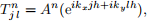
to derive the stability condition for the method:

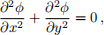
(iii) [2 points] Briely explain a strategy that you could use to obtain a solution to the two-dimensional Laplace equation,
using the FTCS scheme for two-dimensional difusion, Eq. (19).
