关键词 > COMP4702
COMP4702 Report
发布时间:2024-05-17
Hello, dear friend, you can consult us at any time if you have any questions, add WeChat: daixieit
COMP4702 Report
1. Objective
The objective of this report has two parts:
1. Find a good regression problem that can be done on the Rel 2 Nutrient_file dataset.
2. Develop a model that has a high predictive performance on an unseen dataset.
2. Finding a Regression Problem
We first need to understand the dataset and find the features and target for the regression problem. The Rel 2 Nutrient_file dataset has the energy, classification, and nutrient information of 1616 different food examples. It has 293 columns, and 288 of them are of nutrient information. Each of these are for a specific nutrient and specifies a numerical value for each food representing the amount contained in that food. There are 2 columns for energy, one including dietary fibre, and one not.
Since energy is a continuous measurement, it is a good candidate for the target of our regression problem. We will arbitrarily choose the energy with the dietary fibre.
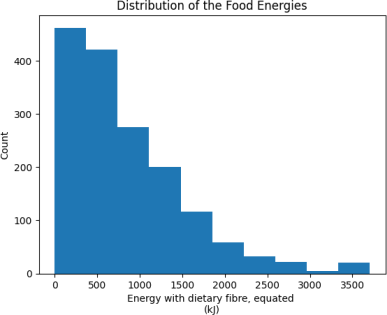
Figure 1. Distribution of Food Energies.
However, the distribution of the energy is skewed, which may make it difficult to evaluate the predictions (see Figure 1). For example, if the error for a particular food was 100kJ, this would be small if the food had 3000kJ of energy but very large if it had 10kJ. To make this easier, we will transform the energy with log(x + 1).
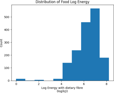
Figure 2. Distribution of Food Log Energy
Figure 2 shows the distribution of the energy with the log transformation. Although this shows some outliers with lower log energy, this is much beter in terms of skewness. We will use this as the target. We will use mean squared error as the evaluation metric – a common choice for regression problems.
Not all the 288 nutrient columns are good candidates for the features of our regression problem. This is because the large number of null values present in the columns. 58 of the nutrient columns have no null values whatsoever in the dataset. We will thus use these 58 columns as the features. 58 columns is a lot, so overfitting is an issue to keep in mind. If the model performance was poor, we can atempt incorporate some of the other columns.
For performance evaluation, we will use an 80-20 training and testing split. The test data will only be used at the end to evaluate our final model as an “unseen dataset”. The test data will not be used to choose our final model or to fine-tune hyperparameters. This is to avoid fitting the model on the test data, which would invalidate the performance evaluation as a measure of performance on unseen data.
3. Selecting the Best Model
To select the best hyperparameters for each model, and to select which model to use as our final model, we will use 10-fold cross validation. These folds are created on the training dataset from the previous 80-20 split. We will compute the train and test MSE losses for each of the 10 iterations. The means of these train and test losses will be referred to as cross-validation train and cross-validation test losses respectively. We will use the cross-validation test loss as the metric to choose the best model and cross-validation train loss to analyse underfitting and overfitting.
We use this method over using a hold-out dataset as it is a more accurate estimation of the model performance, and the models we will look at are not too computationally expensive.
4. Linear Regression
As a baseline model, we will use a simple multivariate linear regression. It achieved a cross-validation train loss of 0.233 and cross-validation test loss of 0.451. We can see that the train loss is lower than test loss, and that is expected.
Figure 3 shows how the test loss varied between each fold of cross-validation. It is quite a big variation. Because linear regression has an analytical exact solution, the variation should be due to the variation in the training and test data in each iteration of cross-validation. This suggests that for a given iteration of cross-validation, the test loss from the hold-out set may not be a good estimate of the true expected error for new data. This supports the use of cross-validation instead of another hold-out set in choosing the best model and hyperparameters.
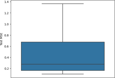
Figure 3: Box plot of the test loss observed for the 10 folds of the cross-validation process.
5. Improving the Model by Regularization
In our linear regression model, there is a gap between the training and test losses. This may be due to overfi![]() ng and may be improved by incorporating regularization techniques.
ng and may be improved by incorporating regularization techniques.
Looking at the coefficients of the final trained linear model, we can see a huge variation in the magnitudes. Plotting them on a log scale (see Figure 4), we see that some are very small (~10^-5) while others are 100k times larger (~10^0). It may be that the scale of the input varies between different columns. We can check this by plotting the distribution of the sample standard deviations of each column (see Figure 5). We see that the variation in the standard deviations is large, which may explain some of the variations in the coefficient magnitudes. To account for this, we can retrain the linear model over the training data with normalised features. Figure 6 shows that even with normalisation, some coefficients have much larger magnitudes than others. This suggests that L2 and L1 regularization can have some effect on the model, which may reduce overfitting.
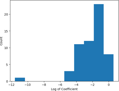
Figure 4: Distribution of the log of non-regularized linear regression coefficients.
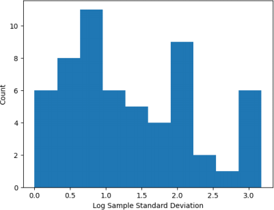
Figure 5: Distribution of the log sample standard deviations of the columns in the training data set.
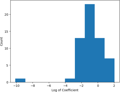
Figure 6: Distribution of the log of non-regularized linear regression coefficients aier normalizing the features. Most coefficients are between the orders of 10^-3 and 10^2.
L2 regularization tends to make coefficients smaller in magnitude because it reduces the regularization term  We also want to normalize features so that the regularization does not affect features with lower values the L2 regularization implemented as Ridge in sklearn. To choose the optimal value on the regularization strength alpha, we will do a search on alpha and find the best performing one. The search on alpha was done on the interval [1, 1000], and the reason is described below.
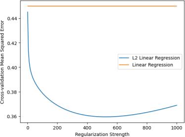
Figure 7: The cross-validation test loss of L2 regularization with different regularization strengths.
Figure 7 shows that the cross-validation test loss achieves a minimum at the strength 523. It Because it looks to keep increasing for greater or lower strengths, we will stop the search here.
Using a strength of 523, the regularized linear regression had a cross-validation test loss of 0.360, suggesting beter generalization performance. This is an improvement from the non-regularized linear regression. Moreover, we can see that the coefficients did get smaller, with values taking orders of 10^-2 or less. (see Figure 8) instead of 10^2 (see Figure 6).
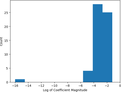
Figure 8: Distribution of L2 linear regression coefficients on a log scale. The coefficients are of order 10^-2 or less.
L1 regularization is another type of regularization that may help the model generalize. It tends to favour sparse coefficients, which may have an impact to the model as it has a large number of coefficients. Unlike L2 regularization, L1 regularization seems to work beter for lower regularization strengths. See Figure 9, which shows that a local minimum of the mean squared error is achieved with strength 0.04.
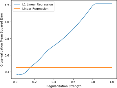
Figure 9: The cross-validation test loss of L1 regularization various regularization strengths. A minimum is reached at strength 0.04.
With the optimal strength of 0.04, the cross-validation test loss was 0.410. This is lower than what was achieved without regularization, but higher than what L2 regularization achieved. Moreover, 19 out of the 58 coefficients were 0, showing that it did make the coefficients sparser.
6. Caveat with Linear Regression
Linear regression works well when there is a linear relationship between the features and the target. For our case, this is likely inaccurate for many of the features, which would lead to the predictions having high bias that contributes to the mean squared error.
We can see how linear the relationships are by looking at the scater plots between Energy and each column values. A subset is shown in Figure 10).
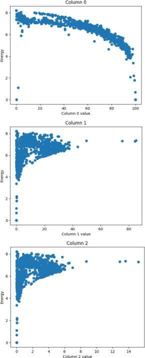
Figure 10: Scaterplot of the Energy over 3 feature values.
They don’t look very linear, so it is possible that more complex models will perform beter than linear regression.
The error metrics also suggest that we may need a more complex model. The cross-validation training losses have not gone below 0.2. It will be difficult for our model to achieve a test error below that without increasing the model complexity. One such model would be a neural network.
7. Neural Network Training Process
To code the neural networks and their training and evaluation processes, we will use pytorch.
Normalization is known to help deep learning models train beter. Because of this, we will normalize the features.
To train the model, we will use a mini-batched gradient-based method to optimize the
training mean square error. Mini-batches are used to help the model avoid overfitting. The Adam optimizer is used which modifies the learning rate based on the curvature of the loss function on top of using the gradient.
In each epoch, we feed all the data into the network and calculate the loss. But because we are using batches, we feed one batch at a time and calculate the loss for each batch. The network weights are updated using the loss and the gradient of the loss calculated for each batch. Pytorch can automatically calculate the gradient using backpropagation.
At the end of each epoch, the model is evaluated on the test data using the same loss function. Both the mean of the train losses for all the batches and the test loss is recorded for the epoch.
This process is repeated for many epochs, ideally until the test loss converges to the minimum. We can analyse how the train losses changes over the epochs to make a guess on when it has converged.
Figure 11 is the code used to do this training process.
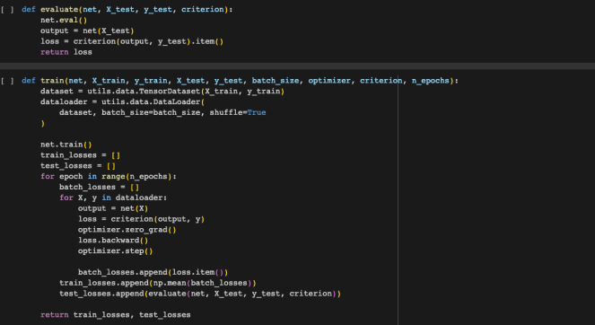
Figure 11: Training and evaluation code.
Like previous models, we will use cross-valida甘on to evaluate this model and fine-tune the hyperparameters. However, sklearn does not support pytorch neural networks for its cross- validation function, so we have to write our own (see Figure 12).
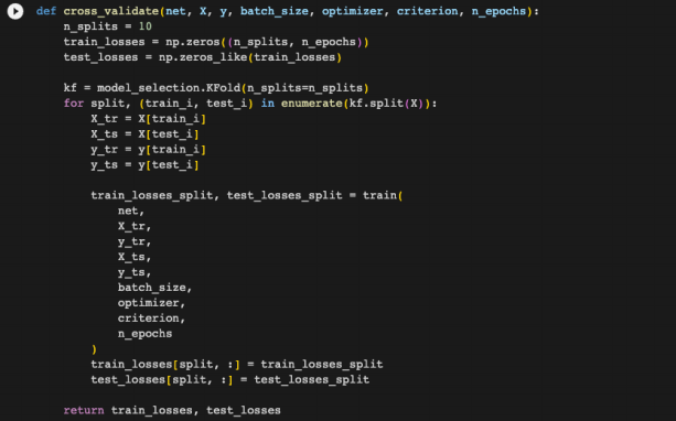
Figure 12: Cross-validation code for pytorch neural networks.
This means the training process is done 10 times, and in each time 9 folds are used as the training data and 1 is used as the testing data. This can take a long time. This means we have less time to do hyperparameter tuning, but this is necessary due to the variation in the test loss we could get for different segmentations of test datasets as we saw when training our linear model.
To analyse how the training and test losses changes over the epochs, we can use the mean loss over all 10 models for each epoch. Aier all epochs have completed, the mean train and test loss over all 10 models would be the cross-validation train and test losses of our final model.
Unlike linear regression, optimizing neural networks oien do not have a closed-form solution. In addition, the complexity of neural networks makes the optimization process non-deterministic, and the results may vary each time it is trained.
8. Single-Unit Neural Network
Unlike previous methods, neural networks require a lot more code to be writen and is more prone to bugs. To test this code, we will train a simple neural net with 1 layer with a single unit and no activation. In theory, this should be equivalent to a simple linear regression.
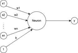
Figure 13: The diagram of a single layer, single unit neural network. The inputs are x1, … ,xn and the prediction output is y. The parameters of the neuron are w1, … ,wn for the weights and b for the bias.
The mathematical model for this simple model (diagram shown in Figure 13) is  = w1x1 + w2x2 + … +wnxn + b. See that this is equivalent to the linear regression model. Thus, if the code is working as expected, it should be possible to achieve similar cross-validation losses to our previous linear model.
Using a batch size of 8, a learning rate of 0.01, and 50 epochs, we achieved a cross-validation train loss of 0.338 and a test loss of 0.377.
These losses are in the same ballpark as what we achieved for our linear model, which was 0.233 and 0.451 for train and test respectively. But they are a bit different.
One possibility for the difference is that the folds used for training the two models will have been different from each other, where each model had different combinations of data points in each fold. However, the training dataset in each cross-validation iteration would be 90% of all the data. It is probably difficult to get much variation in the training data regardless of how the folds are assigned.
Another possibility is that the model’s training loss did not converge to the minimum. This explains the train loss being higher, and different test loss. However, the mean loss over the 10 tests for each epoch seems to have converged (see Figure 14).
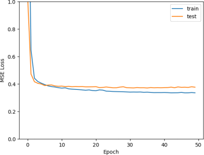
Figure 14: Mean training and test loss over the epoch (mean over 10 cross-validation iterations).
Although the means look converged, perhaps some of the 10 training processes did not converge. We can plot the training loss for each of the 10 training processes (see Figure 15).
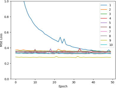
Figure 15: Training loss for each training process over epoch.
We can see that the first iteration starts with a high loss, while all other iterations start with a loss below 0.4. Moreover, the losses for later iterations seems lower than earlier iterations.
This plot can help us realise that in our code for cross validation, we forgot to initialize the weights before the start of each iteration. This means that for each iteration, the model starts with the weights obtained from the result of the previous itera甘on. Moreover, the trend of lower layers having lower training loss suggests that we need to train for more epochs.
By adding the re-initialization and increasing the number of epochs to 200, we get Figure 16.
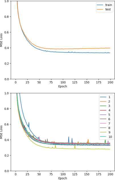
Figure 16: The mean training and test loss (above) and the training loss for each cross- validation iteration (below) for the single-layer neural network.
Now all iterations start with higher training loss. However, the mean train and test losses aier 200 epochs is 0.333 and 0.394 respectively. This is still a bit different from the 0.233 training and 0.451 test losses achieved by our linear model. Moreover, we can see more fluctuations in the loss. It is possible that the loss is not converging to the optimum due to the learning rate being too high. It could also be due to the mini-batch process we used, which computes the gradients from small batches rather than the full dataset which may not be representative of the data.
In addition, the 10 iterations all slightly converge to a different loss, which may be because of the slightly differing makeup of the training and test set in each iteration.
9. Multi-layer Neural Network
To increase the complexity of the model, we will first try a two-layer MLP. The first layer is composed of 30 hidden units, each with ReLU activation. The second layer is the output.
Using a batch size of 8, learning rate of 0.01, and 200 epochs, we get mean train and test scores of 0.107 and 0.209 respec甘vely. This is a significant improvement from our linear models.
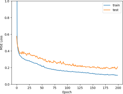
Figure 17: Mean training and test loss over epoch for our two-layer neural network
The mean train losses seem to be flatening out towards epoch 200 (see Figure 17). It is unlikely to have a significantly more decrease, so we do not have to train longer. There is no clear sign of overfitting yet, so the model could be underfitting.
Because of the potential for underfitting, we will further increase the complexity by having 2 hidden layers, each with 30 units. All hidden units have ReLU activation. With all other hyperparameters kept the same as before, we get mean train and test scores of 0.038 and 0.183 respectively.
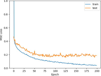
Figure 18: Mean training and testing losses over epoch for our three-layer neural network
The model now seems to be overfitting. The training loss is continuing to go down, while the test loss is staying around 0.2 (See Figure 18).
To help reduce the overfitting while maintaining the complexity needed to achieve low loss, we can incorporate L2 regularization. This is done by adding weight decay. Another method for regularization is to incorporate dropout to each of the layers. With a dropout probability of 0.2 and a weight decay of 0.0001, we got 0.083 training and 0.167 test losses. This is an improvement in the test loss. We can see in Figure 19 that we have less overfitting.
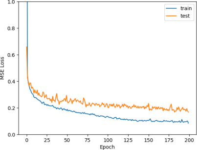
Figure 19: Loss curve for our three-layer neural network with regularization.
We can also try to reduce the complexity a litle bit by lowering the number of units in each layer. We can do a grid search on the values [30, 26, 22, 18]. The lowest cross-validation loss was 0.132 and was observed with 22 hidden units. This is the lowest cross-validation loss we have seen so far.
Running cross-validation again with 22 hidden units, we get a cross-validation test loss of 0.145. This is still lower than all previous models, so we will stick with it. However, it shows how the randomness in the process of initializing and training the neural network leads to the model converging at different local minimums.
10. Evaluation of Final Model
We will use the 3-layer MLP with 22 hidden units in each hidden layer. This is trained on the entire training dataset with the same hyperparameter configurations as we used previously. We then evaluate the network on the hold-out test set that we made at the start.
This results in a test MSE of 0.183. It is slightly higher than our cross-validation losses.
Perhaps this is due to the variation in the dataset as we saw when doing cross-validation, or the randomness in trying to get the model to converge to the global minimum. Regardless, it is a good result and is significantly beter than our baseline linear regression model.
11. Conclusion
In conclusion, we have found a good regression problem to work on and developed a model that has a high predictive performance on the unseen test set. Moreover, we were able to analyse various parts of the models and how they contribute to the models’ prediction performance.
