关键词 > MEC208
MEC208 Instrumentation and Control System S2, 2023-2024
发布时间:2024-05-16
Hello, dear friend, you can consult us at any time if you have any questions, add WeChat: daixieit
Department of Mechatronics and Robotics
MEC208 Instrumentation and Control System S2, 2023-2024
Computer Lab (Lab 2):
Control System CAD and CAS using MATLAB
Introduction
This laboratory work/assignment carries 15% of MEC208 module mark. The work is about learning the engineering software tool to conduct classical control system design and analysis. Among the several options available, MATLAB is chosen as the main software. To help with your learning, the document first sets out the “Examples” that show some of the very typical commands of the Control System toolbox of MATLAB. You are strongly encouraged to practice them yourself and explore other control design functions mentioned in lecture notes and other resources (e.g., the Help Files of MATLAB).
Once you are familiar with the software environment, you can then start to attempt and solve the control problems. You will need to use the theoretical understanding of Classic Control Theory that you acquired so far, and do appropriate problem analysis, mathematical derivation, and deploy suitable numerical tools/functions. At the start of every question, you are encouraged to briefly explain your approach; for sub-parts that need your analysis, please elaborate them concisely.
You are required to submit a well-formatted Lab Report before the deadline (as above). The university’s late submission policy applies to submissions after the deadline. Please refer to LMO module page for the submission steps.
Lastly, and importantly, you are reminded about the university’s academic integrity policy. If you undertake the preparation with other students, or if you use sources from the internet or books, you must acknowledge these in your report by writing a short statement at the beginning of the report.
Aims, Learning Outcomes and Outline
This laboratory work aims to enable the student to:
. Understand the concept of open-loop and closed-loop control systems.
. Understand the mathematical modelling of dynamic systems and different formats of system models.
. Learn computer aided system analysis and design.
. Understand the system stability and how to determine if a system is stable.
Having successfully completed the work, you will be able to:
. Use computer software to assist in dynamical control system design.
. Analyze first- and second-order system responses, and transfer function through Laplace transform.
. Determine system performance and stability with Root Locus Analysis.
. Design feedback controller to stabilize overall system and to meet design specification.
Report Format
The format of the lab/assignment report should be of the following:
. The report should be of single column, font size 11, font style “Times New Roman”. Please be reminded that handwritten reports will NOT be accepted.
. All figures and plots must be clearly labelled.
. In your report, you are expected to explain concisely your approach (i.e., with full sentence and proper grammar, but please avoid unnecessarily long explanation).
. In your answer for each question, do also include all MATLAB code/script that you used to obtain the answers or plots (note: do not separately submit those raw .m files; answer for each question should contain some MATLAB scripts). These codes/scripts should be copied properly into the report and should remain standalone. For example, if you include the code for Question 2a, you must make sure that the codes in this part alone (not linked to other questions) can be copied by the marker into MATLAB for a quick, successful verification.
. For analytical questions, whenever necessary, do also include your analysis and derivation.
Marks will be given on the following basis:
. The 9 questions in the “Computer Lab Work” section carry a total of 100 marks. Each question carries 6 to 16 marks, depending on the complexity of the questions.
. Sub-marks will be awarded to technically correct analyses and comments, MATLAB scripts, mathematical derivation (as necessitated by the questions), graphs/plots (and annotations of the plots), and/or numerical answers. All analysis and comments should have proper sentence structure and correct grammar.
Examples
This part is to introduce about how to start using the Control System Toolbox in MATLAB. You may go through the examples (in this section, and in other online resources) before you start working on the assignment tasks.
Example 1: Input a system described by a transfer function
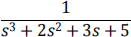
To construct a system model in MATLAB, the command “tf” can be used. For example, to obtain the following input transfer function:
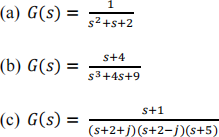
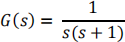
Example 2: Find the system’s zeros and poles
The commands used for this task are “pole” and “zero” . From the signs of system poles, you can determine if the system is stable. For example, given the system G(s):
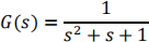
Using MATLAB, the system’s poles can be obtained as follows:
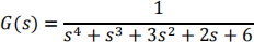
Given another example with system zeros:
Example 3: Obtain the system model in pole-zero format
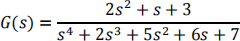
It is at times helpful to control designers to express a system into a form of first/second-order components. For example, given G(s) below, one can express it to pole-zero format as follows:
There are many other control-related numerical tools in MATALB. See some of the listed examples in Part II.
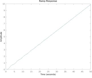
Example 4: Obtain impulse, step, and ramp input responses
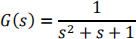
The commands used for obtaining the time responses against unit-step and unit-impulse inputs are, respectively, “step()” and “impulse()” . Taking the following system as the example, its step and impulse responses can be obtained as follows:
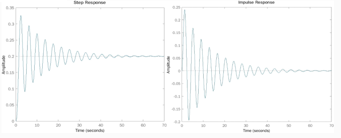
To obtain necessary system ramp input response, the following can be done. Note that the title change is to avoid confusion.
Example 5: Obtain the equivalent/effective transfer function of a closed-loop system
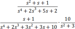
The relevant command is “feedback” . You can obtain the description of this command from MATLAB help, i.e., using command “>>help feedback” . For example, given that a system has a forward-path transfer function G(s)
and feedback-path transfer function H(s)
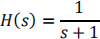
The closed-loop transfer function of the feedback system is obtainable through the following commands:
At this stage of learning, you should be able to obtain the closed-loop transfer function through analytical means. You are encouraged to check whether the numerical tools actually give you the correct answer. At times, through cross-checking, you may find that there are some minor mistakes in your own derivation or MATLAB scripts. You may also attempt the simulation questions at the end of each chapter in the course textbook.
Optional
Before attempting the questions, apart from the numerical tools introduced above, it maybe helpful to you to spend some time understanding other numerical tools/functions (not in any particular order) available to you in the Control System Toolbox of MATLAB.
|
tf step impulse ramp partfrac ilaplace plot feedback series |
pzmap pole zero ss tf2ss lsim expm hold on hold off |
Others (check in MATLAB documentation; there are many more …) |
Computer Lab Work (10 questions)
Problem 1 [6 marks]
Obtain the state variable model/representation for the following transfer functions with unity feedback using your own choice of MATLAB functions:
Problem 2 [8 marks]
Consider the block diagram in Figure P2.
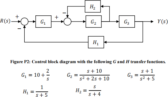
(a) Use an m-file to reduce the block diagram in Figure P2, obtain the equivalent closed-loop transfer function of the above system.
(b) Use the numerical tools available, generate a pole-zero map in the graphical form and calculate the poles and zeros of the closed-loop transfer function. Comment on the overall system stability.
Problem 3 [10 marks]
Consider the system
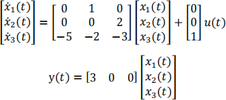
(a) Using the tf function, determine the transfer function Y(S)/u(S).
(b) Assume u(t) is a 10-magnitude pulse input of duration 5 seconds from the start of 0 seconds (and its magnitude becomes zero after that), plot the response of the system with initial condition x(0) = [1 − 2 0]T , for 0 ≤ t ≤ 50.
(c) Then, determine x(t) at t = 20 s for the same initial condition and input as in part (b). Compare and comment on the state and output of the system with the initial condition defined in part (b) for cases with and without the input excitation.
Problem 4 [10 marks]
Consider the closed-loop system shown in Figure P4. The controller gain K can be modified to meet the design specifications.
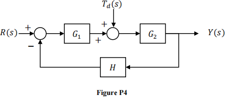
where

(a) Derive the closed-loop transfer function 
(b) Using MATLAB, plot the step response of the closed-loop system for K = 5, 10, and 50. (c) When the controller gain is K = 10, determine the steady-state value of y(t) when the disturbance is a unit step, that is, when Td (S) = 1/S and R(S) = 0.
Problem 5 [16 marks]
Consider the following transfer function:
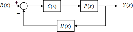
where 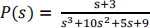 and
and 
(a) Given that C(s) is a continuous-time PID controller with proportional, integral and derivative gains of 1, 5, and 0.1, respectively. Identify the dominant complex poles and complex zeros (if any) of the system. Then, calculate the dominant complex poles ’ natural frequency, damping factor, characteristic rise time (5 to 95%), peak time, percent overshoot and 2% settling time.
(b) Plot and clearly label the unit-step response of Y(s).
(c) Obtain from the figure in part (b) the exact rise time, peak time, percent overshoot, and 2% settling time of the output response. Compare and comment on the difference, if any, between the answers in part (c) and part (a).
Problem 6 [10 marks]
The forward-path of a closed-loop transfer function with unity feedback is given by
(a) Obtain the response of the closed-loop transfer function T(s) to a unit-step input.
(b) Determine the step response of the system after adding zeros at 0, -0.5, - 1.5, and -2.5,
respectively, to G(s). Compare the results with the original step response in part (a), what conclusions can be drawn regarding the effect of adding a zero at different locations with respect to the to a second-order system?
Problem 7 [12 marks]
A magnetically levitated high-speed train travels/floats above its rail system, leaving air gap between them. The train system is depicted graphically in Figure P7(a). The air gap control system has a unity feedback system.
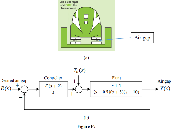
The goal is to select K so that the response for a unit-step input is reasonably damped. Sketch the root locus and select K so that the Ts ≤ 3 s and P. O. ≤ 20%. Determine the actual unit-step response for the selected K. Determine from the plot the settling time and the percent overshoot and explain their difference(s), if any, with the theoretical expectation/calculation.
Problem 8 [12 marks]
Figure P8 shows a closed-loop system with a tunable feedback parameter k, where k is a positive number.
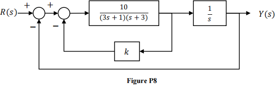
(a) Draw a root locus diagram to reflect the effect of changing k. Then, determine the range of possible k values that can produce a pair of dominant oscillatory/complex poles with the characteristic damping factor more than 0.4 and the characteristic 2% settling time less than 3 s.
(b) Analyze the plot in part (a) and propose the final value of k that can produce a quicker possible response. Then, plot the unit-step response of the output y(t), and comment on the effect of third pole onto the overall behavior of the system.
Problem 9 [16 marks]
As the control engineer in Xiaomi’s electric vehicle (EV) company, you are assigned tasks to analyze and propose a solution to the new model SU7’s linear speed dynamics (note: for simplicity, only one dimension is considered here) with its front and rear wheels powered by two closed-loop controlled interior permanent magnet motors. The overall vehicle linear speed dynamics is depicted graphically in Figure P9. V Tef (s) is the speed reference input, Td is the disturbance input, and V(s) is the vehicle linear speed. You are expected to justify, in the form of textual description, your design solution using the control system understanding from the module (especially the system modelling and control part), mathematical derivation, simulation result, or any other means deemed appropriate.
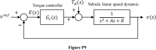
(a) Parameters of the vehicle speed dynamic are estimated, through experiments, as A = 2 and B = 3. Your task is to propose a suitable form of controller Gc (s) that can eliminate the steady-state vehicle speed error due to step input. Explain your answer with sufficient evidence and suggest suitable Gc(s) gain/parameter value(s) to ensure a fast closed-loop response with damping coefficient being in between 0.3 to 0.4 values. Plot the unit-step input response of the closed-loop system.
(b) Later, the company owner requests that the vehicle’s linear ramp performance should be similar to that by Porsche Taycan Turbo S, which achieves 100 km/h from 0 km/h through linear speed ramping (means constant acceleration) at 2.6 seconds. Discuss whether the proposed controller Gc (s) by you in part (a) can fulfill the requirement. Explain and justify your answer with sufficient evidence. Then, propose modification to the proposed controller Gc (s) in part (a) to make it better.
