BusOBA 2321 – Business Analytics Model Building Exercise #1 Summer Semester 2024

Hello, dear friend, you can consult us at any time if you have any questions, add WeChat: daixieit

BusOBA 2321 – Business Analytics

Model Building Exercise #1

Summer Semester 2024

Before you begin, please download excel on your computer. It is provided by the University. Microsoft Excel is needed for this class. Do not use Excel Online, Google Sheets or Apple Numbers  .

To install Microsoft Excel, follow the instructions listed at the following link:

https://support.office.com/en-us/article/Download-and-install-Office-using-Office-365-for-business- on-your-PC-or-Mac-72977511-dfd1-4d8b-856f-405cfb76839c  .

.    Be sure to sign into Microsoft Office using your buckeyemail email. You tuition pays for a Microsoft Office license so that allows you to get excel for free

.    Once excel is downloaded, you can now begin your MBE 1

Please note the following when you submit this assignment and any other MBE:

.    If you are unsure of what a button in excel is called, you can hover over the button with your mouse cursor and the name of the button should appear in a popup

.    If the ‘Aptos’ font is not available in your version of Excel, use the ‘Arial’ font instead

.    If the file you submit has a tilde (~) at the start of the file name, you have submitted the wrong file.

o The tilde (~) at the start of a file name indicates that it is a temporary file that excel uses to save changes while you are working on it and this temporary file can not be opened.

o We cannot grade these files and you will receive a zero for the assignment if it’s submitted

.    When you submit a file to CarmenCanvas, it generates a preview of that file as a PDF

o This is okay, as when the assignment is graded, the grader can see and download the original file that you submitted

o If you would like to check the file format of your submission, follow the instructions below: 

.    Navigate to the CarmenCanvas Dashboard

.    Click on the Icon on the left side of the screen labeled ‘Account’ 

.    Click on the ‘Files’ link

.    Find and Click on the ‘Submissions’ folder

.    Find and Click on the folder for this course, it will have “BUSOBA 2321” in the name 

.    In this folder, you will see every file you submitted to this course and can download them to double check those submission files

Model 1 – Grade Calculator

Objective: Data Visualization – the importance of formatting, spreadsheet layout, and presentation of data. Review of concepts learned in CSE 2111.

Problem Statement: You have just started a new semester and are taking your core Business Analytics course, BusOBA 2321 at the Fisher College of Business. Your professor has become increasingly

distressed that Business Majors cannot figure out the simple algebra involved in calculating their grades   and your first assignment is creating your own grade calculator. To do this, you will be creating a model in Excel where you can input your assignment grades to calculate your current grade and predict your future grade.

Construct the Grade Calculator Model:

1. Open a blank MS Excel file and save it as “BusOBA 2321 - MBE1 Name.#”. We do this so that anyone

using this file easily know what the spreadsheet is and who is the author.

1.1. Replace “Name.#” with your own last name and OSU dot number.

1.2. Save the file somewhere you can access later, such as OneDrive or your computer.

2. Format the worksheet with tab “Sheet 1”

2.1. Left click the box left of column A and above row 1, this selects all the cells in the sheet 2.1.1. The entire sheet will be shaded

2.2. Format the sheet as Aptos, 12 pt

2.2.1. From the “Font” menu, select “Aptos” and “12” 

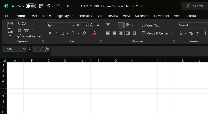
Screenshot 1: Button Locations

3. Label the tab “Grade Calculator”. While not necessary in a simple workbook like this, sheet names help identify sheets in large workbooks, like the ones we will use later in MBE 2.

3.1. Double click the ‘Sheet1’ tab at the bottom left of the screen and replace the word “Sheet1” with “Grade Calculator”

4. Format the Columns and Rows we will use. This step sets up the basic structure of the worksheet. 

4.1. Set the row 1 height 55

4.1.1. Click row 1

4.1.2. With row 1 highlighted, right click to see the context menu

4.1.3. Click ‘Row Height’

4.1.4. Type “55” then press ‘Enter’

4.2. Set every Column’s width to 15, except for Column A which will have a width of 30.00 

4.2.1. To set the column width of every column in a sheet:

4.2.1.1. Select all the cells in the sheet

4.2.1.2. Right click the column letters

4.2.1.3. Select column width

4.2.1.4. Type “15” then press “enter

4.2.2. To set just one column’s width:

4.2.2.1. Click on the column letter of the column you want to adjust

4.2.2.2. Right click that column’s letter

4.2.2.3. Then set the column width

4.3. If your version of Excel does not allow you to set widths and heights to numbers (this is true in some older versions of Excel for Apple products), approximate the widths and heights to be similar to Screenshot 2. 

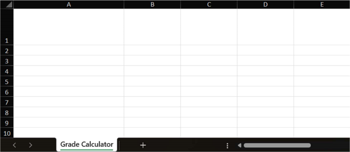
Screenshot 2: Basic Sheet Structure

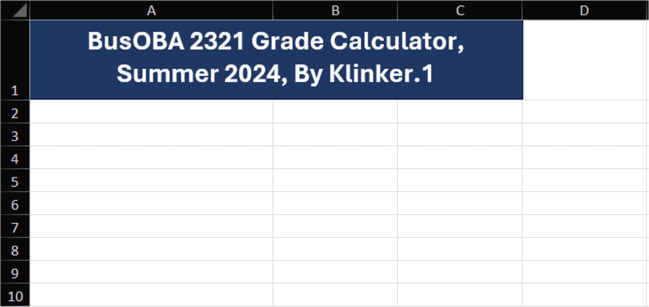
Screenshot 3: Title Block

6. Format the cells. This step sets up the table rows that will calculate your grade.

6.1. Set cells A3 through C7 format to be 14pt, bold, and centered

6.1.1. To select multiple cells at a time, click the starting cell (A3) and while holding down the left click, drag to the ending cell (C7) and release the click. This should form a box around those cells, allowing you to the format for all included cells simultaneously.

6.2. Add borders - borders help the reader to distinguish cells from one another 6.2.1. Add borders to cells C3:C5 and A7:C22

6.2.1.1. To add simple borders to cells

6.2.1.1.1. Select the cells you want to add borders to

6.2.1.1.2. Under the ‘Paragraph’ section, click the dropdown arrow called ‘Borders’ and select ‘All Borders’

6.2.1.1.2.1. OR under the 'Font’ menu, select the icon that looks like a window and, using the pull-down menu, select “All Borders”

6.3. Merge cells A3:B3, A4:B4, and A5:B5.

6.3.1. To merge cells

6.3.1.1. Select the cells you want to merge

6.3.1.2. Under the ‘Alignment’ section, there is a button with two arrows called ‘Merge and Center’, click that button

6.3.1.3. The cells should now appear as one

6.4. Format cells A3 thru A5 as right aligned and indented one unit.

6.4.1. To right align a cell

6.4.1.1. Select the cells you wish to align

6.4.1.2. Under the ‘Alignment’ menu, select the button called ‘Align Right’ 6.4.2. To indent a cell

6.4.2.1. Select the cells you wish to indent

6.4.2.2. Under the ‘Alignment’ section, select the button called ‘Increase Indent’ and press it the desired number of indent units (in this case, once)

6.5. Merge and Center cells A7:C7

6.6. Format cells A8:C8 bold and centered

6.7. Format cells A9:C22 as right aligned with an indent of one

6.8. For cells B9:C22 format the cells to be percents with two decimal places

6.8.1. To format a cell as a percent with two decimal places

6.8.1.1. Select the cells you want to format as a percentage

6.8.1.2. Under the ‘Number’ section, select the ‘%’ button

6.8.1.3. Then click the ‘Increase Decimal’ button twice

6.9. Add thick outside borders to the ranges C3:C5, A7:C7, A8:C8, A9:C13, A14:C18, A19:C20, A21:C22, and B8:B22.

6.9.1. The process is the same as the above border instructions, except you select ‘Thick Outside Borders’ instead of “All Borders’

7. Add color coding so that the reader is clear regarding the type of cell they are observing. We use colors to distinguish between data inputs, calculations, outputs, and key outputs.

7.1. Yellow indicates input data.  Set cells B9:C22 as yellow.

7.1.1. Select cells B9 to C22

7.1.2. Click the ‘Fill Color’ drop down menu in the ‘Font’ section

7.1.3. Select ‘Yellow’ from the ‘Standard Colors’

7.2. Light green indicates formulas.  Set cell C3 as light green.

7.2.1. The process is the same as above, but select ‘Green, Accent 6, Lighter 80%’

7.3. Dark green indicates cells with key outputs – the green indicates a formula cell and the dark

color attracts the reader’s attention to that key output. Set cells C4:C5 as dark green.

7.3.1. The process is the same as above, but select ‘Green, Accent 6, Lighter 50%’

7.3.2. With a dark background, we need to use a light font so that the reader can actually

see the contents of the cell. Set the font of C4 and C5 to white and bold. 7.4. Your model should look like Screenshot 4 

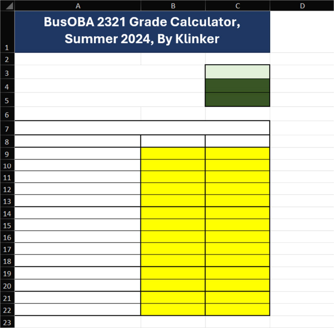
Screenshot 4: Sheet Formatting

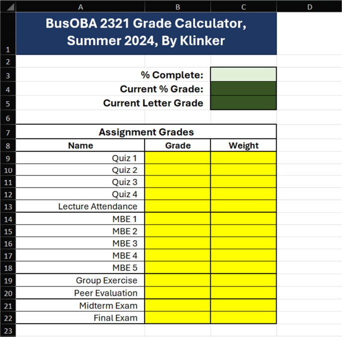
Screenshot 5: Row and Column Titles

9. Create the ‘Grading Scale’ table. The ‘Current Letter Grade’ cell (C5) will reference the ‘Grading Scale’ when reporting the earned course grade.

9.1. Using knowledge from previous steps create a table in cells E7 thru G19, similar to Screenshot 6

9.2. Format the cells as follows:

9.2.1. Cells E9:E19 are left aligned, indented five units

9.2.2. Cells F9:G19 are centered, percentages, with 0 decimal places

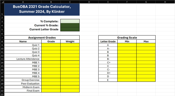
Screenshot 6: Grading Scale Table

10. Enter the formulas to calculate the desired outputs. We won’t be delving into the specifics of what each of these formulae do in this MBE, but each will include detailed explanations in later MBEs (can you feel the excitement?).  Enter or copy each of these equations into the indicated cell without the quotation marks. When copying a formula, it must be pasted in the dialog box (see Screenshot 7) directly under the menu bar, not into the cell.  Otherwise, you will lose your font AND only get a text string rather than a formula.

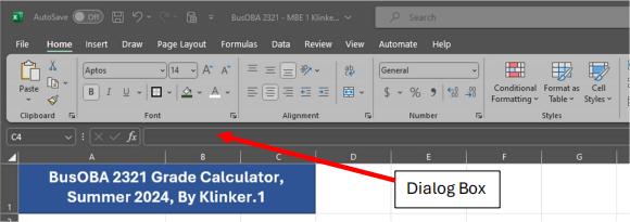
Screenshot 7: Dialog Box Position

10.1. In cell C3 enter or copy the following formula:

“=SUMIF(B9:B22,"<>"&"",C9:C22)-IF(ISBLANK(B13),0,MIN(C9:C13))”

10.2. In cell C4 enter or copy the following formula:

“=ROUNDUP((SUMPRODUCT(B9:B22,C9:C22)-IF(ISBLANK(B13),0,MIN(B9:B13*C9:C13))-

IF(B20,0,B19*0.1*C19))/C3,2)”

10.3. In cell C5 enter or copy the following formula:

“=XLOOKUP(C4,F9:F19, E9:E19,,-1,1)”

NOTE: Cells C4 and C5 will appear to be a “#DIV/0!” error at this stage. That is expected.

11. The Peer Evaluation is a special type of assignment as it does not receive a grade. Failure to turn in the peer evaluation results in a 10% reduction of your individual group exercise score. To simulate  this, we assign the peer evaluation a score of either TRUE or FALSE.  Where TRUE is the peer evaluation being turned in on time and FALSE is the peer evaluation not being turned in on time. We derive a data validation formula to perform this calculation.

11.1. Select cell B20

11.2. Navigate to the ‘Data’ menu

11.3. Under the ‘Data Tools’, select ‘Data Validation’ – a pop-up menu will appear 11.4. Enter the options and values as seen in Screenshot 8

11.5. Then click OK

11.6. There should now be a dropdown menu in cell B20 that allows you to select between the values of TRUE and FALSE

 

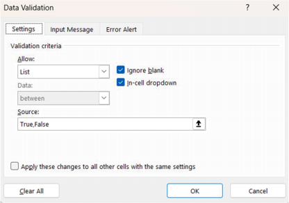
Screenshot 8: Data validation

12.  To complete the model, you must fill out your input cells.

12.1. Much of the information you will need to do this is found in the course syllabus.

12.2. Screenshot 9 shows some of the inputs filled in and the resulting outputs in cells C3:C5.

12.3. Once you have the Grading Scale table complete and all above steps complete, add the following data to your table:

12.3.1. Enter all the course weights (from syllabus) C9 thru C22

12.3.2. Enter 100% for Quiz 1.

12.3.3. Enter 85% for MBE 1.

12.3.4. Set the drop down menu in B20 to ‘True’ and add ‘0’ as the weight in C20.

13. Now, add a watermark to prove that you are submitting your own work. To do this we will start by creating another rectangle shape

13.1. Using the instructions from step 5, create a rectangle shape from B6:E8

13.2. Ensure the box is Aptos Black, font size 40, black color, and bold as the format

13.3. Enter your “First Name, Last Name.#” into the box

13.3.1. For example: “Terry Klinker.1”

13.3.2. If your name doesn’t fit into the box, reduce the font size until it does 13.4. Format the shape by right clicking it and selecting “Format Shape”

13.5. Under the paint bucket shaped tab, select ‘No Fill’ and ‘No Line’

13.6. Under the pentagon shaped tab, select 3-D Rotation and change the z rotation to 45 13.7. Under the ‘Text Options’ options tab, set the transparency to 60%

14. While there are still inputs that need to be filled in, screenshot 9 should help to provide some guidance on how to finish the MBE.  NOTE: SCREENSHOT 9 DOES NOT SHOW THE FINISHED MBE 

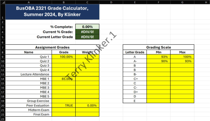
Screenshot 9: Incomplete MBE

And VOILA! You have finished MBE 1! (And there was much rejoicing)

Save your file and submit the spreadsheet via CarmenCanvas.  Make sure the file you submit does not include a tilde (~) at the start of the name. The name of the file you submit should look like this “ BusOBA 2321 MBE 1 Name.#.xlsx” except you should replace “Name.#” with your own last name and OSU dot number.