关键词 > DigitalSignalProcessing
Lab 1: Basic Digital Signal Processing
发布时间:2024-05-13
Hello, dear friend, you can consult us at any time if you have any questions, add WeChat: daixieit
Lab 1: Basic Digital Signal Processing
1. Sketch of concepts
The functions that we will consider represent digital signals. Thus the natural model to present them are sequences of real numbers.
In practice we only have a inite sequence of terms x1 , . . . , xk but to analyze it we may consider it ininite by padding it with ininite zeros before and after it. Sometimes, it is also convenient to consider complex valued sequences although they may have not a physical interpretation.
We are interested in transforming this signal, to eliminate noise from it for instance. The type of transformations that we are going to
consider are linear operators y = T (x),  , i.e
, i.e
T (λx + μz) = λT (x) + μT (z).
This operators are usually denoted in the engineering literature as Lin- ear Systems.
Another important property that allows us to use Fourier Analysis techniques is that we will only consider time invariant linear systems (LTI for short).
Definition 1. A system T is invariant if it commutes with the translations, i.e. T 。τm = τm 。T, where τm is a delay of the sequence: τm (x[n]) = x[n 一 m].
That is, in a LTI “if we delay the input, we delay the output” . If Tx = y then T (τm (x)) = τm (y).
In the following, we will use ininite series but we will not worry about convergence because most of our signals will be compactly sup- ported or very rapidly decaying.
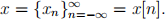
Definition 2. A basic example of discrete signal if the impulse signal δ, this signal is deined as
This is a basic piece because we can express any sequence as a linear combination of delays of the delta function, that is x =:k x[k]τk δ . If we have a linear system, we give a special name as how it responds to the delta function.
Definition 3. Given any linear time invariant system T we deine its impulse response function h as
h = T (δ).
The impulse response function h[n] of an LTI system is very impor- tant because it completely characterizes the system.
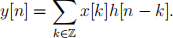
Proposition 1. Given any LTI system T, with impulse response function h, then the system y = T (x) acts as
Proof. We know that for all x, x =Σk x[k]τk δ . Then by linearity
By the time invariance

We recognize immediately the convolution:
Definition 4. Given two signals x, z. We deine its convolution y = x? z = z?x as
This is the complete analogous deinition that we had in the real setting. We have just proved that any LTI system is a convolution operator with the impulse response function. It is a very easy exercise to check that given any impulse response function h (with compact support to avoid problems of convergence) deines an operator by con- volution that is LTI. Thus we have a complete characterization.
1.1. Fourier analysis and LTI. We are going to use Fourier anal- ysis to describe and understand LTI systems.
Definition 5. We deine the Fourier transform of a signal x[n] as a complex valued function X deined on [-π, π].
Observe that we may recover the signal from its Fourier transform as:
Observe that the role of the Fourier coefficients and the function is reversed with the Fourier series that you know.
A signal x[n] is characterized by its Fourier transform X . As the physical signals that we will consider are real valued signals, observe that X(-ω) = (X(ω)).
If a signal x has Fourier transform X with support in (-δ, δ)
[-π, π] near the origin we say that x is a low frequency signal. If the support intersects the complement suppX \ ([-π, π] / (-δ, δ)), we say that x has high frequency content.
Let us see that the complex valued signals x[n] = eiωn , for some ixed ω 2 [-π, π] are the eigensequences of any LTI system T with response function h.
We know that y = T (x) = x?h. That is
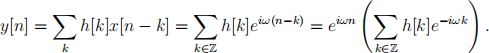
If we denote by H(ω) the Fourier transform of the impulse response
function h[n], i.e., H(ω) =Σk2Z h[k]e-iωk , we obtain
y[n] = T (x[n]) = H(ω)x[n].
That means that x[n] is an eigenfunction of the TLI system with eigenvalue H(w). Therefore all TLI system “diagonalize” through the Fourier transform. If we know how the system acts against the expo- nentials, we know the eigenvalues H(ω) and therefore we know h[n] which describes the system.
This can also be seen by the convolution theorem.
Theorem 1. If we have signals y, x,h such that
y = x? h
and Y (ω), X(ω), H(ω) are its corresponding Fourier transforms, then
Y (ω) = H(ω)X(ω)
Proof. We compute the Fourier transform of y:
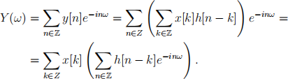
We make the change of variables m = n - k and we get
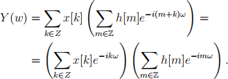
That is Y (ω) = X(ω)H(ω).
Thus one can interpret H(ω), the Fourier transform of the impulse response function h[n], as the spectral multiplier of the LTI system. It is usually called the frequency response of the LTI system. If jH(ω)j is very small for some values of ω 2 [-π, π] then the system T attenuates the frequencies of a signal x at that frequencies. A low pass system is a system such that jH(ω)j is small for big w and a high pass system has frequency response small for small values of ω .
For many applications the relevant signal is low-frequency and the high frequency components are due to noise. Thus it is interesting to construct low pass ilters to eliminate the noise from the signal.
Exercise 1. Take a look at the data compiled by el Departament de Salut of new infections by COVID-19 in Catalunya since March 1, 2020. I have extracted the total data (without segregation by sex or age) in the fle “newcases.txt” Observe that the daily data is very noisy. In some graphic representations widely used they have opted to reduce the noise by drawing a curve using points obtained by taking a fve day moving average of the data. That is they replace x[n] by y[n] = (x[n - 2] + x[n - 1] + x[n] + x[n + 1] + x[n + 2])/5 and draw a curve passing through the new points y[n] to observe the trend.
. Express the new data y[n] as a convolution against some im- pulse response function h, y = x?h.
. Compute and draw the absolute value of the Fourier transform of the flter h.
. Try to explain why the noise is reduced. You can either plot the Fourier transform of use the Octave/Matlab command freqz to analyze it.
. Propose alternative flters h.
Exercise 2. Eliminate the noise from a GPS, signal. Take the heights obtained from a GPS from one of the stages of the circuit “Car- ros de Foc” . Concretely from the stage from Refugi Ventura Calvell to Estany Llong. You can get the original fle here. I have parsed the heights and they are in the fle heights.txt.
. Compute the total height climbed and descended, that is com-pute
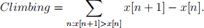
and
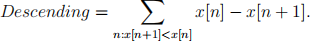
where x[n] is a vector that contains the heights that you should have read previously.
. Apply a low pass flter, i.e. remove part of the noise produced by errors in the GPS measurement. For this you can try tofnd the coefficients h[n] of a low pass flter such that its Fourier transform mimics a characteristic function. Alternatively you can use a flter as in the previous exercise.
. Recompute Climbing and Descending once we have applied a low pass flter.
. Explain the diference.
