ECON0051: ECONOMICS OF REGULATION SUMMER TERM 2024

Assessment Component: Sample paper for 70% Remote Online Controlled Condition Examination

Time allowance: You will have 2 hours to complete the actual examination, plus additional collation time of 20 minutes and an Upload Window of 20 minutes. The additional collation time has been provided to cover any additional tasks that may be required when collating documents for upload, and the Upload Window is for uploading and correcting any minor mistakes. The additional collation time and Upload Window time allowance should not be used for additional writing time.

If you have been granted SoRA extra time and/or rest breaks, your individual examination duration and additional collation time will be extended pro-rata and you will also have the 20-minute Upload Window added to your individual duration.

If you miss the submission deadline during the 40-minute Late Submission Period and do not receive approved mitigation for the circumstances relating to your late submission, a Late Submission Penalty will be applied by the Module Administrator.  At the end of the Late Submission Period, you will not be able to submit your work via Moodle and you will not be permitted to submit work via email or any other channel.

All work must be submitted anonymously in a single PDF file. Do not write your name and student number in either the file or the filename. Your answer file must be named: ECON0051FinalExam.pdf.

Page Limit:  12 pages A4.

Additional instructions: Please note that the general goal of any assessment in Economics is to test students’ ability to analyse and evaluate economic problems, so that students can reach considered and appropriate conclusions, and can competently communicate the reasoning behind these conclusions. Therefore, the present open book examination will also assess your clarity of expression, your ability to set out an argument or answer clearly and logically, as well as the overall structure and presentation of your answers (including referencing, where appropriate).

Academic Misconduct:  By submitting the actual ECON0051 assessment, you will be confirming that you have not violated UCL’s Assessment Regulations relating to Academic Misconduct contained in Section 9 of Chapter 6 of the Academic Manual.

Number of Questions Answered Policy: In cases where a student answers more questions than requested by the examination rubric, the policy of the Economics Department is that the student’s first set of answers up to the required number will be the ones that count (not the best answers). All remaining answers will be ignored.

Questions

You must  answer a total of TWO  questions.  Answer  ONE question from Part A  and ONE question from Part B.

All questions have the same weight overall (marks for each subquestion are stated within each question) .

PART A

Answer ONE question from Part A:  either Question A1 or Question A2.

A1. A monopoly company has the following cost function: C(Q) = 15Q + 400, and faces an inverse linear demand function: P(Q) = 100 − Q.

(a)  [5 points] Is this company a natural monopoly?  Explain your answer providing a diagram and relevant calculations.

(b)  [10 points] What is the deadweight loss associated with this monopoly business?  Explain your calculations and use diagrams to illustrate your answer where relevant.

(c)  [10 points] The regulator has decided to mimic the outcome of competition and therefore sets price equal to marginal cost.  Do you think this is a good idea?  Why/why not?  Use calculations and diagrams to support your answer where relevant.

(d)  [25 points] What price would you suggest that the regulator sets?  Make clear your assump- tion on the regulator’s objective(s). Explain how the price would be calculated and why it is the best price to use. Support your answer with calculations, diagrams.

A2.  Suppose a monopolist produces two services, 1 and 2.  Further suppose the firm’s total cost (in British Pounds) of supplying q1  units of service 1 and q2  units of service 2 is:

c(q1 , q2 ) = 1800 + 20(q1  + q2 ) .

Suppose the demand functions for the two services are, respectively:

q1  = 100 − p1

q2  = 120 − 2p2

(a)  [10 points] If the regulator of the monopolist set the price of each service equal to marginal cost, what prices would prevail? And what profit-level would these prices generate for the monopolist?

Then suppose the regulator raises the marginal cost price of each service by the same proportion x until the firm’s total revenue is equal to total cost. Compute these increased prices and the corresponding quantities sold.

(b)  [40  points] Suppose now that the regulator, who is fully informed of the monopolist’s demand functions, proposes a Ramsey pricing scheme.  Describe briefly what Ramsey prices are and then compute the Ramsey prices and the corresponding quantities (assuming the firm breaks even).   Justify your answer by checking second-order conditions.   Compare the welfare loss (relative to marginal cost pricing) of the Ramsey prices with that of the proportionally raised marginal cost prices from part (a). Interpret your findings!

PART B

Answer ONE question from Part B: either Question B1 or Question B2.

B1.  Consider the liberalization of an industry in which an incumbent monopolist is currently subject to quantity regulation (as in the regulation model with demand uncertainty studied by Basso, Leonardo J., Nicol´as Figueroa, and Jorge V´asquez (2017):  “Monopoly Regulation under Asymmetric Information: Prices versus Quantities”, The RAND Journal of Economics, Vol.  48, No. 3, pp. 557–578).

In particular, the monopoly firm has private information about consumer demand, as captured by a parameter θ ∈ [−10, 10]. The inverse demand function is P (q, θ) = 100 + θ − 10/1q where θ is a demand shock parameter.  The firm observes θ, which is its private information, while the regulator does not. However, the regulator has a prior belief about θ captured by a cumulative distribution function G (θ) with density g (θ) ≡ G′ (θ) = 20/1. The firm’s cost function is C (q) = 40q.

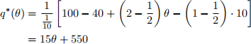
Under  the  regulator’s  expected  welfare-maximizing  incentive  compatible  quantity-regulation mechanism  {q∗ (θ), T∗ (θ)}θ∈[0,1]   (as  derived in Tutorial 4 - you do  not  have  to  repeat  this derivation here), in which the firm’s profits receive a weight of α = 2/1 ) the firm is asked to produce an output quantity:

(a)  [20 Points] Use the information above to compute the numerical value of expected social welfare W under the optimal quantity-regulation mechanism {q∗ (θ), T∗ (θ)}θ∈[0,1](you do not have to repeat the derivation of the expression for W from Tutorial 4).  Then compute the welfare loss from asymmetric information by comparing this level of expected social welfare  W to the one that would obtain in the first-best if the regulator observed the realization of θ just like the firm.

(b)  [15 Points] Now suppose the industry is liberalized without any further quantity regulation. A second firm with identical technology enters the market and competes in quantities with the original firm (Cournot competition). Both firms have the same cost function and both know the true realization of the demand shock  and therefore  face the inverse demand function is P (Q) = 100+θ − 10/1Q, where Q = q1 +q2 and qi , i = 1, 2, is the output quantity of firm i.

What is the industry equilibrium (price, output, firm profits, and social welfare) when the two companies compete in a single time-period by announcing simultaneously how much output they will sell? How does the expected social welfare under Cournot competition in the liberalized industry compare with the expected social welfare under quantity regulation of the monopoly firm in part (a)?

(c)  [15 Points] Finally, show that the possibility of collusion between the two firms may further reduce the welfare from liberalization of the industry. To this end, (for simplicity) assume θ = 0 so that inverse demand is P = 100 − 10/1Q and assume furthermore that the firms compete over an infinite horizon, discounting future profits at a rate of δ ∈ (0, 1].  What discount rate would be sufficient for them to sustain a collusive outcome? You can assume that the collusive agreement takes the following form:  firms set collusive prices as long as both firms have played the collusive strategy in the previous period.   If  either firm deviates, both firms resort to producing the competitive quantities (from part (i)) in all future periods.

B2.  Consider the following simple version of the regulation model with demand uncertainty studied by Basso, Leonardo J., Nicol´as Figueroa, and Jorge V´asquez (2017):  “Monopoly Reg- ulation under Asymmetric Information: Prices versus Quantities”, The RAND Journal of Eco- nomics, Vol. 48, No. 3, pp. 557–578.

In particular, the monopoly firm has private information about consumer demand, as captured by a parameter θ  ∈  [0, 1].   The  inverse  demand function is  P (q,θ)  =  a + θ − bq  where  θ  is a demand shock parameter.  The firm observes θ, which is its private information, while the regulator does not. However, the regulator has a prior belief about θ captured by a cumulative distribution function G(θ,γ) with density g (θ,γ) ≡ G′ (θ,γ) = γ (1 − θ)γ−1  for γ  ≥ 1.  The firm’s cost function is C (q) = cq with c > 0.

The regulator wishes to design an incentive compatible and expected welfare-maximizing quantity- mechanism which (as derived in Tutorial 4 - you do not  have to repeat this derivation here)  consists of a non-decreasing assignment rule q (θ) ∈ R+  and a lump-sum transfer rule T (θ) ∈ R where:

Such a menu {q (θ), T (θ)}θ∈[0,1] induces truthful revelation by the firm for all realizations of θ . The regulator chooses the details of this menu so as to maximize the expected value of social welfare, which is given by the weighted sum of net consumer surplus and the firm’s profit, where a weight of α ∈ [0, 1] is applied to firm profits:  CS (q (θ)) − T (θ) + αΠ(θ). The regulator must also account for the firm’s particiation constraint: Π(θ) ≥ 0 for all θ ∈ [0, 1].

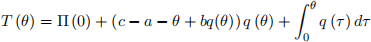
(a)  [10  points]  Use the above information about the incentive compatible transfer schedule T (θ) to express the regulator’s expected social welfare in terms of the assignment schedule q (θ), demonstrating that it takes the form:

Then maximize W  pointwise to obtain the optimal assignment schedule  q∗ (θ) and the optimal profit-level Π(0) of the lowest type.

(b)  [30  points]  How  do the regulated price and quantity schedule change if the regulator’s belief about the firm’s demand becomes less ‘favourable’ in the sense that it considers lower demand shocks more likely (Hint:  an increase in the parameter γ shifts more probability mass of the distribution g (θ,γ) towards lower realizations of the demand shock θ).  What happens in the limit as γ becomes arbitrarily large? Interpret your findings!

(c)  [10  points]  Compare  the  optimal  quantity schedule  q∗ (θ)  with the first-best regulation mechanism (the one that would be used by the regulator it the firm’s type θ was observable, as described by Definition 2 in Basso et al.  (2017)).  Explain why you think the optimal schedule q∗ (θ) distorts the firm’s output quantity downwards, and especially so for low realizations of the demand shock θ?  In particular, discuss the incentive problem that would arise if a firm with private information about its type θ were asked by the regulator to produce the first-best quantity qFB (θ).