MA117 Programming for Scientists: Project 2 Root Finding

发布时间：2024-05-11

Hello, dear friend, you can consult us at any time if you have any questions, add WeChat: daixieit

MA117 Programming for Scientists: Project 2

MA117 Project 2: Root Finding

Administrative Details

• This project is the second of the three assignments required for the assessment in this course. Details of the method of the submission via the Moodle system have been described in the lecture notes and are also available on the course web page.

• This assignment will count for 35% of your total grade in the course.

• The automated submission system requires that you closely follow instructions about the format of certain files; failure to do so will result in the severe loss of points in this assessment.

• You may work on the assignment during the lab session, provided you have completed the other tasks that have been set. You can always use the work areas when they are not booked for teaching. If you are working on the assignment on your home system you are advised to make regular back-up copies (for example by transferring the files to the University systems). You should note that no allowance will be made for domestic disasters involving your own computer system. You should make sure well ahead of the deadline that you are able to transfer all necessary files to the University system and that it works there as well.

• Remember that all work you submit should be your own work. Do not be tempted to copy work; this assignment is not meant to be a team exercise. There are both human and automated techniques to detect pieces of the code which have been copied from others. If you are stuck, then ask for assistance in the lab sessions. TAs will not complete the exercise for you, but they will help if you do not understand the problem, are confused by an error message, need advice on how to debug the code, require further explanation of a feature of Java or similar matters.

• If you have more general or administrative problems e-mail me immediately. Always include the course number (MA117) in the subject of your e-mail.

1 Formulation of the Problem

Finding the roots of a function is a classical and extremely well-known problem which is important in many branches of mathematics. In Analysis II, you have probably seen that it is often easy to prove results about the existence of roots. For example, using the Intermediate Value Theorem, you should easily be able to prove that the function f(x) = x − cos x has a root in the interval [0, 1]. On the other hand, calculating an exact value for this root is impossible, since the equation is transcendental.

Root finding is a classic computational mathematical problem, and as such there are many algorithms which one may use to approximate the roots of a function. In this project, you will write a program which uses the Secant algorithm. Let f ∶ ℂ → ℂ be continuously differentiable and pick two points z, z1 ∈ ℂ. Consider the sequence of complex numbers generated by the difference relation

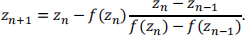
Typically, if zn converges and , then f(z∗) = 0.

Some methods of finding the roots (Newton-Raphson) require knowing the derivative off. Whilst there are numerical tricks to accomplish this, this problem is somewhat beyond the scope of this course. Instead, you will use the Secant method which does not require the derivative, however it does require two initial values. We will consider a polynomial P ∈ ℂ[z]; i.e.

Where ak ∈ ℂ.

1.1 Secant Fractals

One of the most fascinating aspects of this problem arises from a very simple question: given two starting positions z0, z1 ∈ ℂ, which root does the sequence produced by Secant converge towards? It turns out that the answer to this question is very hard!

Figure 1 shows two examples of how we might visualise this for the polynomial f(z) = z3 − 1. Recall that the roots of this polynomial are for k = 1,2,3 (i.e. the third roots of unity). Each of the three colours represents one of these roots. In the left-hand figure, we colour each point depending on which root the method converges to. The right-hand figure is the same, asides from the fact that we make the colour darker as the number of iterations it takes to get to the root (within a tolerance ε) increases. The resulting images are examples of fractals, which you have undoubtedly seen before.

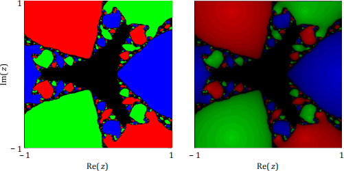
Figure 1: An example of fractals for the function f(z) = z3 − 1 in the square with bottom left-corner −1 − i and width 2.

Don’t worry if all of this seems quite difficult – the main aim of the assignment is for you to successfully implement the Secant scheme. Most of the code to deal with drawing and writing the images will be given to you.

1.2 Summary

Your task then involves several distinct elements. You will:

. write a class to represent complex numbers

. write a class to represent a polynomial in ℂ[z]

. implement the Secant method to find the roots of the polynomial

. investigate some interesting fractals and plot some pictures!

2 Programming instructions, classes in your code and hints

On the course web page for the project, you will find the following files, which should serve as templates and should help you to start with the project. As with the previous projects, the files have some predefined methods that are either complete or come with predefined names and parameters. You must keep all names of public objects and methods as they are in the templates. Other methods have to be filled in correctly and it is up to you to design them properly. Where a method returns a value, a placeholder will exist to return zero or an empty class. The files define three basic classes for your project:

. Complex.java: represents points z ∈ ℂ;

. Polynomial.java: represents polynomials in ℂ[z];

. Secant.java: given two initial Complex points z, zଵclose to the root calculate the corresponding root of Polynomial by Secant, if possible;

• Project2.java: will generate a fractal similar to the one pictured above in a square.

These classes are documented in more detail in the following sections. You should complete them in the order of the following sections, making sure to carefully test each one with a main function.

2.1 Complex

Complex is the simplest of the classes you will need to implement and will represent complex numbers. In fact, it bears a striking resemblance to the CmplxNum class you (hopefully) implemented in week 14.

They are not identical however, so you should carefully when incorporating your solution to that into this new class.

2.2 Polynomial

The Polynomial class is designed to represent a polynomial 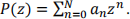As such, it contains coeff, an array of Complex coefficients which define it. It is assumed that coeff[0] corresponds to a0, coeff[1] to a1 and so forth. To complete this class, you will have to:

1. Define appropriate constructors. There are two that need implementation; a default constructor which initialises the polynomial to the zero polynomial (i.e. a0 = 0), and a more general constructor which is passed an array of Complex numbers {a0, a1, … , an} which should be copied into coeff. In addition, you should ensure that if any of the leading co-efficients are zero then they are not copied. For example, if the constructor is passed the complex numbers {a0, a1, 0, 0} then it should copy{a0, a1} to coeff. (When testing for equality to zero, do not use any tolerances.)

2. Return the degree of the polynomial. Recall that degf = N.

3. Evaluate the polynomial at any given point z ∈ ℂ. Note that you should not implement a pow function inside Complex as it is unnecessary and inefficient. Instead, notice that (for example)

2.3 Secant

This class will perform the Secant algorithm. There are two constants defined in this class:

• MAXITER: the maximum number of iterations to make; that is, you should generate the sequence z for 0 ≤ n ≤ MAXITER and no more.

• TOL: At each stage of the Secant algorithm, we must test whether a sequence converges to a limit. In this project, we will say that zM approximates this limit if, at any stage of the algorithm, |zM − zM-1| < TOL and |f(zM)| < TOL . We then say that the starting points z0, z1 required M iterations to converge to the root.

Additionally, you will need to define the iterate function. This accepts two parameters, z2, z1, which defines the initial condition of the Secant difference relation, and performs the root finding algorithm. There are three things that can occur during this process:

• everything is fine and we converge to a root (OK)

• the difference |f(zn) − f(zn-1)| goes to zero during the algorithm (ZERO)

• we reach MAXITER iterations (DNF)

If any of the last two cases occur, then you set the error flag err to be ZERO and DNF respectively; otherwise, err is set to OK. Here is a quick example of how Secant should be used:

Complex[] coeff = new Complex[] { new Complex(-1.0,0.0), new Complex(),

new Complex(), new Complex(1.0,0.0) };

Polynomial p = new Polynomial(coeff);

Secant n = new Secant(p);

n.iterate(new Complex(), new Complex(1.0, 1.0));

System.out.println(n.getRoot());

This will print out the root off(z) = z ଷ − 1 obtained with the starting point z = 0, zଵ = 1 + i.

2.4 Project2

Project2 will be responsible for drawing images of the fractals we saw in Figure 1. However, let us briefly consider how images are represented on computer first. A two-dimensional image is, in general, broken down into small squares called pixels. Each of these is given a colour, and there are generally many hundreds of pixels comprising the width and height of the image.

An example of this can be seen in Figure 2. This image (badly) represents a square in the complex plane with top-left corner −1 + i and bottom-right corner 1 − i. In Project2 you will generalise this concept to visualise squares with a top-left corner origin and width width, stored as instance variables inside Project2. The image will be of size NUMPIXELS by NUMPIXELS. Each pixel can be accessed by using an ordered pair (j, k) where j is the row number, k the column number and (0,0) is the top left pixel, with 0 ≤ j, k < NUMPIXELS. The image itself will be generated using createFractal, which accepts a single argument colourIterations. When true, the function generates a figure like the right-hand side of Figure 1.

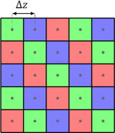
Figure 2: A 5x5 pixel image representing the square with top left corner −1 + i and bottom right corner 1 − i. The centre of each pixel represents a complex number on the plane.

To complete the class,first ensure that you call the setupFractal function at the end of your constructor. This will initialise the more complex drawing objects. It also checks that the polynomial you have given it has 3 ≤ degp ≤ 5 . You will not need to consider any other polynomials in this class. Then inside createFractal, use the following logic:

1. Copy colourIterations to the instance variable.

2. Iterate over each pixel at position (j, k). Then translate this position to a complex number using pixelToComplex, which uses the simple mapping (j, k) ↦ OTigin + Δz(j − ik). NOTE: Δz is the distance between two pixels being plotted in the complex plane.

3. Use 0 and this complex number as the starting points to run through the Secant algorithm.

4. Check to see whether you’ve found this root already. You will store the list of already found roots inside the ArrayList roots. The index function will return the position of a root in the roots. In this formulation, two complex numbers z1 and z2 are equal if |z1− z2| < Secant. TOL.

5. Finally, colour the pixel using the colourPixel function using the root’s index in the array for the rootColour.

After you are done, you can save the image using saveFractal. Here is an example from start to finish, which creates the two images of Figure 1. Note that your filename should end with .png:

Project2 f = new Project2(p, new Complex(-1.0,1.0), 2.0);

f.createFractal(false);

f.saveFractal("fractal-light.png");

f.createFractal(true);

f.saveFractal("fractal-dark.png");

You should then create a document which is precisely one page long. In this document, pick a polynomial P(z), a square in the complex plane and use your program to generate the two plots. You should call this file Fractal.pdf and ensure it is saved as a PDF file.

3 Submission

You should submit, using the Moodle system, the following four files: Complex.java, Polynomial.java, Secant.java, Project2.java and Fractal.pdf which contains your plots.

There will be a large number of tests performed on your classes. This should allow for some partial credit even if you don’t manage to finish all tasks by the deadline. Each class will be tested individually so you may want to submit even a partially finished project. In each case, however, be certain that you submit Java files that compile without syntax error. Submissions that do not compile will be marked down.

If you submit a code and later (before the deadline) you realise that something is wrong and you want to correct it, you may do so. You can submit as many versions as you wish until the deadline. However, only the last submission will be tested. Each new submission replaces the previous one, so in particular, you MUST submit all files required for the project even if you corrected only a single file.

Keep back-up copies of your work. Lost data are not a valid excuse for missing the deadline.