关键词 > ENG5009
ENG5009 Advanced Control 5
发布时间:2024-05-11
Hello, dear friend, you can consult us at any time if you have any questions, add WeChat: daixieit
ENG5009 Advanced Control 5
Laboratory Document
Overview
This lab exercise introduces the Fuzzy Logic Toolbox within MATLAB, introduces the robot model and simulation to be used in the assignment and allows you to create and test a simple Neural Network.
You will be required to work your way through the examples provided and keep track of your progress using the answer grid provided on Moodle. This answer grid is to be included as an appendix in the final assignment report and is worth 20% of the assignment mark.
Laboratory 1
Introduction
The main purpose of this first lab is to provide you with an introduction to the Fuzzy Logic Toolbox within MATLAB. This is achieved through:
• The MATLAB Fuzzy Logic Toolbox Tutorial,
• Implementing the Fuzzy Logic system you developed into the command line,
• Create a second Fuzzy Logic system.
Following this process will give you the necessary skills to create a Fuzzy Logic system.
1. Introduction to Fuzzy Logic Toolbox
The first stage in this tutorial is to learn more about the fuzzy logic toolbox in MATLAB.
The easiest way of doing this is to follow the Mathworks Tutorial, which can be found here:
https://uk.mathworks.com/help/fuzzy/building-systems-with-fuzzy-logic-toolbox-software.html
This tutorial introduces you to the basics of using the toolbox. The skills you learn developing this system will support you with the main assignment – if you choose to use a Fuzzy logic controller.
Using the standard settings, provide the tipping level for the following input values in Table 1.
Table 1: Service and Food Values
|
Service |
Food |
|
5 |
5 |
|
7 |
8 |
|
10 |
2 |
Note these values in the Laboratory answer sheet.
Change the defuzzificiation method to the Mean of Maximum and using the values in Table 1 note the values in the Laboratory answer sheet. To change the defuzzification method return to the front page of the Fuzzy Logic toolbox and change via the drop down menu on the right hand side of the screen.
Change the defuzzificiation method to the Bisector and using the values in Table 1 note the values in the Laboratory answer sheet.
2. Integrating the Fuzzy system into the command line
To use the Fuzzy system developed you need to be able to call it from within a MATLAB script. Ensure you have reset the tipper FIS back to Centroid defuzzification before saving your values.
To use tipper in the command line, do this:
tipper = readfis('tipper'); % create a variable name and assign your fis file to it
You then evaluate the inputs using the following:
tip = evalfis(tipper, [5 5]); % @outputs =
evalfis(@nameofFIS,@inputs)
Further information on the integration of the FIS into the command line, or script file, can be found here:https://uk.mathworks.com/help/fuzzy/evalfis.html. Note the tipping value within the
Laboratory Answer Sheet for the inputs in Table 2, using the command line method.
Table 2: Service and Food Values
|
Service |
Food |
|
6 |
3 |
|
2 |
2 |
|
10 |
7 |
3. Further Fuzzy Logic Example
Create a fuzzy logic system for an AC system based on the following parameters.
• Input range: 5 to 32
• Output range: -20 to 20
• Defuzzification method: Centroid
The input fuzzy sets are defined in Table 3 and the output fuzzy sets are defined in Table 4 and the rules are supplied in Table 5.
Table 3: Input Fuzzy Sets
|
Fuzzy Set |
Type |
Parameters |
|
Too Cold |
Trapezoid |
[4 5 12 14] |
|
Cold |
Trapezoid |
[12 14 16 18] |
|
Comfortable |
Trapezoid |
[16 18 22 24] |
|
Warm |
Trapezoid |
[22 24 26 28] |
|
Hot |
Trapezoid |
[26 28 32 35] |
Table 4: Output Fuzzy Sets
|
Fuzzy Set |
Type |
Parameters |
|
High power cool |
Trapezoid |
[-22 -20 -12 -8] |
|
Low power cool |
Trapezoid |
[-12 -8 -6 -2] |
|
off |
Trapezoid |
[-6 -2 2 6] |
|
Low power warm |
Trapezoid |
[2 6 8 12] |
|
High power warm |
Trapezoid |
[8 12 20 22] |
Table 5: Rules
|
If |
Then |
|
Too Cold |
High power warm |
|
Cold |
Low power warm |
|
Comfortable |
off |
|
Warm |
Low power cool |
|
Hot |
High power cool |
Using the system you have developed, note the values in the Laboratory Answer Sheet based on the inputs in Table 6.
Table 6: Inputs for the AC system
|
Input Temperature, °C |
|
9 |
|
13.1 |
|
26.5 |
|
20 |
This completes Laboratory 1.
Laboratory 2
For the assignment you will be using a model of a four wheeled robot. This model will be available from the ENG5009 Moodle page under the Lab and Assignment section.
This laboratory provides a demonstration of how to use the robot model and simulation that is to be used and how to integrate a controller within it.
The model is called: DynamicalModel.m and is fully described in
ENG5009_ModelDescription_2024.
In addition, there is a simple simulation file, RunModel.m, that can be used to run the model.
Further files that maybe of interest are:
drawrobot.m: this file draws a representation of the robot on to a given figure.
WallGeneration.m: supports the development of obstacles.
Sensor.m: A function that provides a forward-looking sensor that returns the nearest objects on the right and left handside of the robot.
1. Basic Operation
The first stage is to learn how to use the model and the simulation file.
Apply the voltages in Table 7 to voltage_left and voltage_right.
Table 7: Values to be applied to left and right Motors
|
Voltage Left, V |
Voltage Right, V |
Expected Action |
|
6 |
6 |
Forward motion |
|
-6 |
6 |
Rotation Left |
|
6 |
-6 |
Rotation Right |
For each of these insert the output plot figure 1 into the Laboratory Answer Sheet.
2. Basic Manoeuvre
You are required to move the robot:
• a short way forward,
• turn left,
• a short way forward,
• turn right manoeuvre,
• a short way forward.
The output should be like the path shown in Figure 1 below. When completed insert output Figure 2 into the Laboratory Answer Sheet.
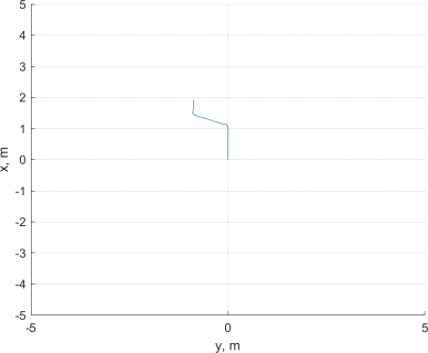
Figure 1: Path of robot
To achieve this, you need to create a simple time-based controller that alters the voltage_left and voltage_right values as and when required. For example, you could use several if statements to alter the variables at relevant time steps. For example, the code below will alter the voltage_left and voltage_right after 1s.
if (time(timeStep) >= 1)
voltage_left = -6;
voltage_right = 6;
end
3. Running the Model with a Fuzzy Controller
Develop a fuzzy controller that allows the robot to avoid obstacles. This should be based on the example developed during Lectures 5 and 6 of the course. You should use the Matlab Fuzzy Logic Toolbox to do this.
For this you will be required to add in obstacle detection. To do this add the following line:
[sensorOutput] = Sensor(robot_x, robot_y, headingAngle, obstacleMatrix)
You will also be required to draw walls on the plot. To do this, set drawWalls to 1.
Insert figure 2 into the Laboratory Answer Sheet.
4. Running the Model with a Neural Controller
In lectures 7 and 8 we discussed avery simple Neural network controller that should be able to drive the robot forward while avoiding obstacles.
The first stage is to create a neural network controller based on Figure 2 below and using the values
calculated in the lecture for each of the weights. Insert the MATLAB output Figure 2 into the Laboratory Answer Sheet. Comment on the behaviour of the system.
Given the output provided, make a change to the system to improve the output. Detail the change you made in the Laboratory Answer Sheet and provide the MATLAB output Figure 2.
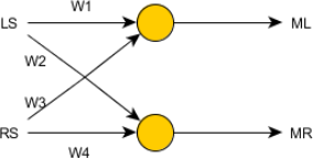
Figure 2: Simple Neural Network
To create the Neural network it is advised to use code similar to that below:
sumN1 = (weight(1)*sensorOutput(1) + weight(3)*sensorOutput(2));
sumN2 = (weight(2)*sensorOutput(1) + weight(4)*sensorOutput(2));
if (sumN1 > weight(5))
voltage_left = 3;
else
voltage_left = 0;
end
if (sumN2 > weight(6))
voltage_right = 3;
else
voltage_right = 0;
end
