ESE 605-001: Modern Convex Optimization Spring 2022 Final exam

Hello, dear friend, you can consult us at any time if you have any questions, add WeChat: daixieit

ESE 605-001: Modern Convex Optimization

Spring 2022

Date: May 2022

Final exam

This is a 24 hour take-home final. Please turn it in on Gradescope within 24 hours of your respective start times. The exam is open textbook, open notes, and open homework, and you may cite equations from the book, notes, and homework. You may also refer to online documentation for CVX* and your programming language of choice. Any other outside or online resources are strictly prohibited.

There are six problems on this exam. All problems have equal weight, but we will only count the best five out of six questions towards your final exam grade. Some are (quite) straightforward. Others, not so much. Be sure you are using the most recent version of CVX, CVXPY, or Convex.jl.

You may not discuss the exam with anyone until May 7th, 6PM EST, after everyone has taken the exam. The only exception is that you can ask the teaching staff for clarification, via e-mail – please do not use Piazza so as to avoid accidentally sending a public post that was meant to be private. We have made the exam as unambiguous and clear as possible, so we are unlikely to say much.

Assemble your solutions in order (problem 1, problem 2, problem 3, . . . ), starting a new page for each problem. Put everything associated with each problem (e.g., text, code, plots) together; do not attach code or plots at the end of the final.

We will deduct points from long, needlessly complex solutions, even if they are correct. Our solutions are not long, so if you find that your solution to a problem goes on and on for many pages, you should try to figure out a simpler one. You do not have to LATEXyour solutions, but we do expect neat, legible exams from everyone.

When a problem involves computation you must give all of the following: a clear discussion and justifi- cation of exactly what you did, the source code that produces the result, and the final numerical results or plots. Remember, the more information and explanation that you give us regarding your thought process, the easier it is for us to give you partial marks!

Files containing problem data can be found as ProbX.mat and ProbX.* files here:

https://www.dropbox.com/sh/osll885kp5ejutw/AACiWgdrpG2ZVXzUE5i7_Qx-a?dl=0

For problems asking you to generate random data and do not specify what random seeds to use, please use the following random seeds:

• Matlab: randn(’state’,0); rand(’state’,0);

• Python: np.random.seed(0)

• Julia: Random.seed!(0);

1. In this question you will implement a barrier method for solving the standard form LP

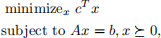
with variable x ∈ R n, where A ∈ R m×n, with m < n. Assume that A is full rank, and that the sublevel sets {x | Ax = b, x 0, cT x ≤ γ} are bounded for all γ ∈ R.

(a) Implement Newton’s method for solving the centering problem

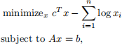
with variable x, given a strictly feasible starting point x0. Your code should accept A, b, c, and x0, and return the primal optimal point x ? , a dual optimal point ν ? , and the number of Newton steps executed. Use the block elimination method to compute the Newton step.

Plot the Newton decrement λ 2/2 versus iteration k, for problem data and initial points as specified below to verify that your implementation gives asymptotic quadratic convergence. As stopping criterion, you can use λ 2/2 ≤ 10−6 . Set the algorithm parameters for backtracking line-search as α = 0.1 and β = 0.5.

To generate the random problem data A, b, c, and x0, follow the following approach. You will perform two trials with m = 20 and n = 100, i.e., run the experiments and create the required plots twice, once for each of the two problem instances generated as described next.

Generate data for the first trial using random seed “0”, and data for the second trial using random seed “1.” First, generate A randomly by drawing Aij i.i.d. from a standard normal distribution N (0, 1). Then generate a random positive vector x0 by drawing (x0)i i.i.d. from a standard uniform distribution U[0, 1], and then set b = Ax0. This ensures that x0 is strictly feasible. The parameter c can be chosen randomly by drawing ci i.i.d. from a standard normal distribution N (0, 1). To be sure the sublevel sets are bounded, set the values of the last row of A to their absolute values (such that this row has only positive entries).

Hints:

• You should check that your computed x ? and ν ? (nearly) satisfy the KKT conditions of the problem.

• We recommend computing λ 2 using the formula λ 2 = −∆x T nt∇f(x). You don’t really need λ for anything; you can work with λ 2 instead. (This is important for reasons described below.)

• There can be small numerical errors in the Newton step ∆xnt that you compute. When x is nearly optimal the computed value λ 2 = −∆x T nt∇f(x) can actually be (slightly) negative. If you take the square-root to get λ, you’ll get a complex number and your line search will never exit. However, this only happens when x is nearly optimal. So if you exit on the condition λ 2/2 ≤ 10−6 , everything will work as expected even when the computed value of λ 2 is negative.

• For the line search, make sure that enough iterations have been run so that x + t∆xnt > 0.

(b) Using the centering code from part (a), implement a barrier method to solve the standard form LP

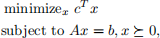
with variable x ∈ R n, given a strictly feasible starting point x0. Your LP solver should take as argument A, b, c, and x0, and return x ? . You can terminate your barrier method when the duality gap, as measured by m/t, is smaller than 10−3.

Check your LP solver against the solution found by CVX*, for the two problem instances generated in part (a) for parameter values of µ = {2, 10, 100}, i.e., for each of the two problem instances generated in part (a), apply the barrier method three times, once for each value of µ.

Plot the progress of the algorithm showing duality gap (on a log scale) on the vertical axis, versus the cumulative total number of Newton steps (on a linear scale) on the horizontal axis.

Your algorithm should return a 2 × k matrix history, (where k is the total number of centering steps), whose first row contains the number of Newton steps required for each centering step, and whose second row shows the duality gap at the end of each centering step. In order to get a plot that looks like the ones in the book (e.g., figure 11.4, page 572), you should use the following code in Matlab

[xx, yy] = stairs(cumsum(history(1,:)),history(2,:));

semilogy(xx,yy);

and in Python

plt.step(np.cumsum(history[0]), history[1])

plt.yscale("log")

plt.show()

(c) Using the code from part (b), implement a general standard form LP solver, that takes arguments A, b, c, determines (strict) feasibility, and returns an optimal point if the problem is (strictly) feasible.

You will need to implement a phase I method, that determines whether the problem is strictly feasible, and if so, finds a strictly feasible point, which can then be fed to the code from part (b).

You can use the code from part (b) to implement the phase I method.

To find a strictly feasible initial point x0, we solve the phase I problem

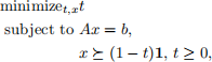
with variables x and t. If we can find a feasible (x, t), with t < 1, then x is strictly feasible for the original problem. The converse is also true, so the original LP is strictly feasible if and only if t ? < 1, where t ? is the optimal value of the phase I problem.

We can initialize x and t for the phase I problem with any x0 satisfying Ax0 = b, and t0 = 2 − mini(x0)i . (Here we can assume that min(x0)i ≤ 0; otherwise x0 is already a strictly feasible point, and we are done.) You can use a change of variable z = x+ (t−1)1 to transform the phase I problem into the form in part (b).

Check your LP solver against CVX* on the two feasible examples from parts (a) and (b), and then generate an infeasible instance using the example of part (a) by setting Aij = |Aij | and bi = −|bi | such that A is element-wise positive, and b is element-wise negative, and verify that your LP solver returns “infeasible”.

2. Consider the problem

with variable x ∈ R n, and data A ∈ S n, b ∈ R n. We do not assume that A is positive semidefinite, and therefore the problem is not necessarily convex. In this exercise we show that x is (globally) optimal if and only if there exists a λ such that

From this we will develop an efficient method for finding the global solution. The conditions (2) are the KKT conditions for (1) with the inequality A + λI 0 added.

(a) Show that if x and λ satisfy (2), then f(x) = infz L(z, λ) = g(λ), where L is the Lagrangian of the problem and g is the dual function. Therefore strong duality holds, and x is globally optimal.

(b) Next we show that the conditions (2) are also necessary. Assume that x is globally optimal for (1). We distinguish two cases.

(i) If ||x|| 2 < 1, show that (2) holds with λ = 0.

(ii) If ||x|| 2 = 1, first prove that (A + λI)x = −b for some λ ≥ 0. (In other words, the negative gradient −(Ax + b) of the objective function is normal to the unit sphere at x, and points away from the origin.) You can show this by contradiction: if the condition does not hold, then there exists a direction v with v T x < 0 and v T (Ax+b) < 0. Show that f(x+tv) < f(x) for small positive t > 0.

It remains to show that A + λI 0. If not, there exists a w with w T (A + λI)w < 0, and without loss of generality we can assume that w T x = 0. Show that the point y = x + tw with t = −2w T x/wT w satisfies ||y|| 2 = 1 and f(y) < f(x).

(c) The optimality conditions (2) can be used to derive a simple algorithm for (1). Using the eigenvalue decomposition A = P ni=1 αiqiqi T , of A, we make a change of variables yi = qi T x, and write (1) as

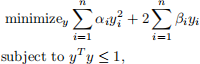
where βi = qi T b. The transformed optimality conditions (2) are

k yk 2 ≤ 1, λ ≥ −αn, (αi + λ)yi = −βi , i = 1, . . . , n, λ(1 − kyk 2) = 0,

if we assume that α1 ≥ α2 ≥ · · · ≥ αn. Give an algorithm for computing the solution y and λ.

Note that you do not have to implement the algorithm.

3. This problem concerns the braking and thrust profiles for an airplane during take-off. For simplicity we will use a discrete-time model. The position (down the runway) and the velocity in time period t are pt and vt, respectively, for t = 0, 1, . . . ,. These satisfy p0 = 0, v0 = 0, and pt+1 = pt + hvt, t = 0, 1, . . . , where h > 0 is the sampling time period. The velocity updates as

vt+1 = (1 − η)vt + h(ft − bt), t = 0, 1, . . . ,

where η ∈ (0, 1) is a friction or drag parameter, ft is the engine thrust, and bt is the braking force, at time period t. These must satisfy

0 ≤ bt ≤ min{Bmax, ft}, 0 ≤ ft ≤ Fmax, t = 0, 1, . . . ,

as well as a constraint on how fast the engine thrust can be changed,

|ft+1 − ft| ≤ S, t = 0, 1, . . . .

Here Bmax, Fmax, and S are given parameters. The initial thrust is f0 = 0. The take-off time is Tto = min{t| vt ≥ Vto}, where Vto is a given take-off velocity. The take-off position is Pto = pTto , the position of the aircraft at the take-off time. The length of the runway is L > 0, so we must have Pto ≤ L.

(a) Explain how to find the thrust and braking profiles that minimize the take-off time Tto, respecting all constraints. Your solution can involve solving more than one convex problem, if necessary.

(b) Solve the quickest take-off problem with data

h = 1, η = 0.05, Bmax = 0.5, Fmax = 4, S = 0.8, Vto = 40, L = 300.

Plot pt, vt, ft, and bt versus t. Comment on what you see: is use of the breaks necessary? How about if we make the runway longer? Report the take-off time and take-off position for the profile you find.

4. Consider the (symmetric, linear phase) finite impulse response (FIR) filter described by its frequency response

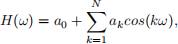
where ω ∈ [0, π] is the frequency. The design variables in our problems are the real coefficients a = (a0, . . . , aN ) ∈ R N+1, where N is called the order or length of the FIR filter. In this problem we will explore the design of a low-pass filter, with specifications:

• For 0 ≤ ω ≤ π/3, 0.89 ≤ H(ω) ≤ 1.12, i.e., the filter has about ±1dB ripple in the ‘passband’ [0, π/3].

• For ωc ≤ ω ≤ π, |H(ω)| ≤ α. In other words, the filter achieves an attenuation given by α in the ‘stopband’ [ωc, π]. Here ωc is called the filter ‘cutoff frequency’.

It is called a low-pass filter since low frequencies are allowed to pass, but frequencies above the cutoff frequency are attenuated.

For parts (a)–(c), explain how to formulate the given problem as a convex or quasiconvex optimization problem.

(a) Fix ωc and N and maximize the stopband attenuation, i.e., minimize α.

(b) Fix N and α and minimize ωc, i.e., we set the stopband attenuation and filter length, and seek to minimize the ‘transition’ band between π/3 and ωc.

(c) Fix ωc, and α, and find the smallest N that can meet the specifications, i.e., we seek the shortest length FIR filter that can meet the specifications.

(d) Use CVX* to find the shortest length filter that satisfies the filter specifications with ωc = 0.4π and α = 0.0316, corresponding to -30dB attenuation. For this subproblem, you may sample the constraints in frequency, which means the following. Choose K = 500 and set ωk = kπ/K, k = 0, . . . , K. Then replace the specifications with

• For k with 0 ≤ ωk ≤ π/3, 0.89 ≤ H(ωk) ≤ 1.12.

• For k with ωc ≤ ωk ≤ π, |H(ωk)| ≤ α. Plot H(ω) versus ω for your design.7

5. We consider a financial system with n financial entities or agents, such as banks, who make payments to each other over discrete time periods t = 1, 2, . . . . We let ct ∈ R n + denote the cash held at the beginning of time period t, where (ct)i is the amount held by the ith entity in dollars.

We let L ∈ R n + ×n denote the liability between the entities at the beginning of time period t, where (Lt)ij is the amount in dollars that entity i owes entity j. You can assume that (Lt)ii = 0, i.e., the entities do not owe anything to themselves. Note that Lt1 is the vector of total liabilities of the entities, i.e., the total amount owed to other entities, and L Tt 1 is the vector of total amount owed to the entities by others, at time period t.

We let P ∈ R n + ×n denote the amount paid between each entity during time period t, where (Pt)ij is the amount, in dollars, paid from entity i to entity j. Thus Pt1 is the vector of total cash payments made by the entities to others in period t (i.e., (Pt1)i is the total payments from entity i to all other entities), and Pt T 1 is the vector of total cash received by the entities from others in period t.

The liabilities and cash follows the dynamics

Lt+1 = Lt − Pt, t = 1, 2, . . . ,

ct+1 = ct − Pt1 + Pt T 1, t = 1, 2, . . . .

Each entity cannot pay more than the cash it has on hand, so we have the constraint

Pt1 ct, t = 1, 2, . . . .

We are given the initial cash held c1 and the initial liabilities L1. You can assume that for each entity, the cash held plus the cash owed to it are at least as much as the amount it owes, i.e., c1−L11+L T1 1 0.

(a) Explain how to find the minimum T for which there is a feasible sequence of payments P1, . . . , PT −1 that results in LT = 0. (Reducing the liabilities to zero is called clearing them.) Your method can involve solving a reasonable number of convex problems.

(b) Carry out your method from part (a) on the data given in Prob5.*.

6. A finite dimensional approximation of a quantum mechanical system is described by its Hamiltonian matrix H ∈ S n. We label the eigenvalues of H as λ1 ≤ · · · ≤ λn, with corresponding orthonormal eigenvectors v1, . . . , vn. In this context the eigenvalues are called the energy levels of the system, and the eigenvectors are called the eigenstates. The eigenstate v1 is called the ground state, and λ1 is the ground energy. The energy gap (between the ground and next state) is η = λ2 − λ1. By changing the environment (say, applying external fields), we can perturb a nominal Hamiltonian matrix to obtain the perturbed Hamiltonian, which has the form

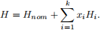
Here Hnom ∈ S n is the nominal (unperturbed) Hamiltonian, x ∈ R k gives the strength or value of the perturbations, and H1, . . . , Hk ∈ S n characterize the perturbations. We have limits for each perturbation, which we express as |xi | ≤ 1, i = 1, . . . , k. The problem is to choose x to maximize the gap η of the perturbed Hamiltonian, subject to the constraint that the perturbed Hamiltonian H has the same ground state v1,nom (up to scaling, of course) as the unperturbed Hamiltonian Hnom. The problem data are the nominal Hamiltonian matrix Hnom and the perturbation matrices H1, . . . , Hk.

(a) Explain how to formulate this as a convex or quasiconvex optimization problem. If you change variables, explain the change of variables clearly.

(b) Carry out the method of part (a) for the problem instance with data given in Prob6.*. Give the optimal perturbations, and the energy gap for the nominal and perturbed systems. The data Hi are given as a cell array; Hi gives Hi .