关键词 > Econometrics

Econometrics Problem Set 2

发布时间：2024-05-10

Hello, dear friend, you can consult us at any time if you have any questions, add WeChat: daixieit

Econometrics

Problem Set 2

Assignment instructions

. You must submit your work via the Turnitin link on moodle by 16:00 on Friday April 19, 2024

. This assignment will be marked for the course assessment and will be worth 10%of your final mark. You must attach your Stata do-file to your answers and failure to do so will result in a zero mark for the computing questions.

. Name, student number, course title, tutorial group number and tutor’s name should be clearly included in the submission. Your answers including Stata do-file should not exceed 8 pages. The Assignment is based on the material covered in both lectures and tutorials up to the end Week 10.

. The assignment is INDIVIDUAL work. You may discuss the assignment with your peers, but you must submit YOUR OWN answers.

. If the answer requires some mathematical calculation show the steps, don’t just report the final results.

. This assignment has a total of 100 points awarded.

. All submissions may be checked for plagiarism. The University regards plagiarism as a form of academic misconduct and has very strict rules regarding plagiarism. For UNSW policies, penalties, and information to help you avoid plagiarism see:

https://student.unsw.edu.au/plagiarism as well as the guidelines in the online ELISE tutorials for all new UNSW students: http:/subjectguides.library.unsw.edu.au/elise. To see if you understand plagiarism, do this short quiz:

https://student.unsw.edu.au/plagiarism-quiz

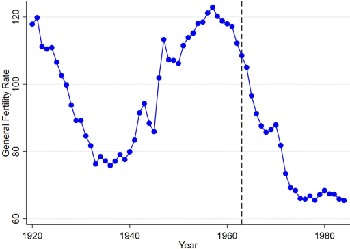
The general fertility rate (gfr) is the number of children born to every 1,000 women of child- bearing age. In this study, we explore the determinants of gfr using three datasets.

The first dataset comprises a time series of gfr in the United States from 1920 to 1984. Drawing on the methodology outlined in Whittington, Alm, and Peters (1990), we apply the following regression equation for our analysis:

gftt = β0 + β1pet + β2 ww2t + β3pillt + ut (1)

The explanatory variables include the average real dollar value of the personal tax exemption (pe); a technology shock variable (pill), which is assigned a value of 1 starting from 1963 to reflect the availability of the birth control pill for contraception; and a macroeconomic environment shock variable (ww2), set to 1 for the years 1941 to 1945, corresponding to the period of the United States' involvement in World War II.

The descriptive statistics of these variables are presented in Table 1.

Table 1: Descriptive Statistics

Variable	Unit	Time span	Mean	Std. Dev.	Min	Max
gft		1920- 1984	92.83	18.72	65.4	122.9
pe	dollar	1920- 1984	110.24	61.57	14.91	243.83
pill		1920- 1984	.34	.48	0	1
ww2		1920- 1984	.08	.27	0	1

1. (10 points) Using OLS to estimate equation (1). Report the results in equation or tabular form. Interpret the estimated coefficients of β1, β2, and β3 .

2. (16 points) An econometrician argues that, for both biological and behavioral reasons, decisions to have children would not immediately result from changes in the personal exemption (pe). Therefore he proposes to use a finite distributed lag (FDL) model of order

gftt = β0 + β1pet + β2pet− 1 + β3pet−2 + β4 ww2t + β5pillt + ut (2)

Using OLS to estimate equation (2). What is the long-run propensity (LRP) of the tax exemption on the fertility rate? Propose a regression equation to perform a t-test on the significance of the LRP and perform the test. What do you conclude from the result of this test (use 5% significance level)?

3. (14 points) Another econometrician analyzing a time series presented in Figure 1 argues that Model (1) is misspecified due to an observable linear time trend in the variable of interest post- 1957. The concern is that omitting a control for this time trend could introduce bias into the estimates. Do you agree with this statement. If you agree with the econometrician's critique, identify the likely direction of bias in the coefficient for the “pill ” variable and provide a rationale for your conclusion.

Figure 1: Time trend of the general fertility rate in the US

The second dataset comprises cross-sectional data for a sample of 4,361 women born between the years 1934 and 1961. This dataset is analyzed to shed light on individual women’s birth decisions. The dependent variable in this analysis is the number of children each woman has had (children), with the major explanatory variables being the years of education (educ) and the age of the women at the time of the interview. Additionally, to account for varying perspectives on childbirth across different age groups, we segment the sample into four cohorts ( C1 − C4 ) based on the women ’s birth years, with each cohort encompassing a span of six birth years (for instance, C1 dummy corresponds to those born in 1934-1940).

We consider a regression of the number of children with respect to females’ education level, age, and the three cohort dummies as follows:

We run OLS regression on Equation (3), and obtain the following regression results:

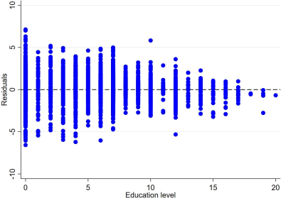
4. (15 points) We analyze the residuals obtained from the regression and use Figure 2 to illustrate the relationship between the residuals and the education level. Based on this visual analysis, identify any potential issues with regression (3). Conduct appropriate statistical tests to verify if Model (3) exhibits this problem, using a 5% significance level. What conclusions can be drawn from the outcomes of these tests?

Figure 2: Relationship between residuals and education level

5. (10 points) Model (3) includes dummy variables for different cohorts. Why has the associated dummy variable for the first cohort C1 been excluded? Using the regression results of Model (3), interpret the coefficients of each cohort dummy.

6. (10 points) Perform statistical tests to determine whether cohort dummies jointly statistically significantly affect the number of children at the 5% significance level. What conclusions can be drawn from this analysis?

To obtain the causal impact of birth control pill’s introduction on the fertility choice, we use a third data set, which is a retrospective longitudinal data set for women born in 1934-1947. These women were asked to recall, for each year from 1958 to 1967, whether they gave birth to a child (newborn). Additionally, we include a variable indicating access to birth control pills by age 16 (buypill). Therefore, the birth control pill was only effective for those who had access to it during the child-bearing ages (buypill = 1). We consider the

7. (15 points) Write down the population equation for those buypill = 1 and buypill = 0 separately. Interpret the coefficient of the interaction term.

8. (10 points) In this retrospective data, the dependent variable (newbornit) variable may have been measured with some errors as respondents could inaccurately recall specific years of childbirth. However, those errors from bad memory are completely at random. How do you think this issue can affect the OLS estimations?