Materials Informatics

Hello, dear friend, you can consult us at any time if you have any questions, add WeChat: daixieit

Materials Informatics – Fall 2021

Problem Set 3

Problems:

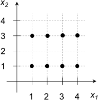
1. For the data set below, find all possible solutions of the K-means algorithm (using different starting points) for K = 2 and K = 4. What if K = 3?

Hint: look for center positions that are invariant to the E and M steps.

2. Show that the M-step equations for estimating the parameters of the Gaussian-Mixture model can be obtained via the following informal optimization process. Assuming that the cluster memberships are known and fixed:

(a) Find the values that maximize the log-likelihood L, and plug in current esti-mates of other quantities.

Hint: use differentiation.

(b) Using the mean estimates in the previous step, find the values that maximize the log-likelihood L, and plug in current estimates of .

Hint: use differentiation.

(c) Find the values that maximize the log-likelihood L.

Hint: This necessitates a slightly more complex optimization process than in the pre-vious two steps, involving Lagrange multipliers, due to the constraints ≥ 0 and  = 1.

The E-step corresponds simply to updating the cluster membership estimates given the estimates obtained in the M-step.

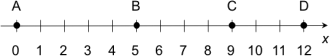
3. Compute manually the dendrograms corresponding to single-linkage, complete-linkage, and average-linkage pairwise cluster dissimilarity metrics for the data below. What do you observe in the comparison among the dendrograms?

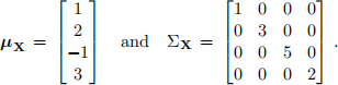
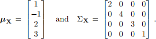
4. Obtain, by inspection, the first and second PCs Z1 and Z2 as a function of X = (X1, X2, X3, X4) and the percentage of variance explained by Z1 and Z2 in the following cases.

(a)

(b)

Coding Assignment:

This assignmemt uses a data set on Fe-based nanocrystalline soft magnetic alloys, which is available from the Book Website. See this reference for more information:

Wang, Y., Tian, Y., Kirk, T., Laris, O., Ross Jr, J. H., Noebe, R. D., Keylin, V., and Arroyave, R. “Accelerated design of Fe-based soft magnetic materials using machine learning and stochastic optimization,” Acta Materialia, 194:144—155.

This data set records the atomic composition and processing parameters along with several different electromagnetic properties for a large number of magnetic alloys. In this project, we will use unsupervised learning to correlate the atomic composition features and the aneealing temperature processing parameter to the magnetic coercivity of the material. Larger values of coercivity mean that the magnetized material has a wider histeresis curve and can withstand larger magnetic external fields without losing its own magnetization. By constrast, small values of coercivity mean that a material can lose its magnetization quickly. Large-coercivity materials are therefore ideal to make permanent magnets, for example.

(a) (Data preprocessing.) The features are the atomic composition percentages (first 25 columns of the data matrix) and the annealing temperature (column 26), while the response vatiable is the magnetic coercivity in A/m (column 34). Preprocessing consists of the following steps:

1. read the spreadsheet into python;

2. discard all features (columns) that do not have at least 5% nonzero values;

3. discard all entries (rows) that do not have a recorded coercivity value (i.e., discard NaNs).

4. add zero-mean Gaussian noise of standard deviation 2 to all feature values (but not the response variable). Do not be concerned with possible negative values. To ensure reproducible results, set numpy’s random seed to zero (execute np.random.seed(0) prior to generating the noise).

5. normalize all feature vectors to have zero mean and unit variance.

Note that the order in which the operations are applied matter. Step 4 is necessary to introduce a small degree of randomness to the data. Step 5 is necessary because the fea-tures are measured on different scales (percentage for the atomix composition and Kelvin for the annealing temperature); in addition, most of the alloys have large Fe and Si composition percentages. Without normalization, Fe, Si, and the annealing temperature would unduly dominate the analysis.

Hint: normalize the data using the StandardScaler function in the sklearn.preprocessing module.

(b) Run PCA on the resulting 741 × 12 feature data matrix.

Hint: use the PCA function in the sklearn.decomposition module.

(c) There are 12 principal components. Plot the percentage of variance explained by each PC as a function of PC number (this is called a “scree” plot. Now plot the cumulative percentage of variance explained by the PCs as a function of PC number. How many PCs are needed to explain 95% of the variance?

Hint: use the attribute explained_variance_ratio_ and the cusum() method.

(d) Obtain scatter plots of the first few PCs against each other (PC1 vs. PC2, PC1 vs. PC3, and PC2 vs. PC3). In order to investigate the association between the features and the coercivity, categorize the latter into three classes: “low” (coercivity ≤ 2 A/M), “medium” (2 A/M < coercivity < 8 A/M), and “high” (coercivity ≥ 2 A/M). Color code the previous scatter plots using red, green, and blue to identify high, middle, and low coercivity. What do you observe? If you had to project the data down into just one PC, while retaining maximum discrimination, which one would it be?

(e) Print the “loading” matrix W (this is the matrix of eigenvectors, ordered by PC number from left to right). The absolute value of the coefficients indicate the relative importance of each original variable (row of W) in the correponding PC (column of W). Identify which two features contribute the most to the discriminating PC you identified in the previous item and plot the data using these top two features. What can you conclude about the effect of these two features on the coercivity? This is an application of PCA to feature selection.