ECON 320: MACROECONOMIC THEORY II

Hello, dear friend, you can consult us at any time if you have any questions, add WeChat: daixieit

ECON 320: MACROECONOMIC THEORY II

ASSIGNMENT THREE

FALL 2021

1. In this question, we add uncertainty into the example economy from Question One on Assignment Two. Recall the description of that economy.

The household has h = 100 units of time and the household’s preferences over consumption of clocks and leisure is given by the following utility function:

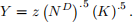
The firm that produces clocks uses household labour and a fixed amount of capital equal to K = 16 with the following production function:

Here z randomly fluctuates between and

At the beginning of each quarter, the household and the firm receive an announcement stating how severe global supply chain (GSC) disruptions will be during that quarter. The announcement can be either very severe or not severe. (I realize this doesn’t quite fit the description of clock production here but global supply chain disruptions are very current so let’s go with it.)

Each quarter, the household and the firm choose labour supply and labour demand after receiving the announcement regarding GSC disruptions but before observing z. They cannot change labour input after observing z but the wage and output can adjust after z is observed.

The household and the firm know that the probability of a particular z occurring in a quarter is related to the severity of GSC disruptions:

(1.A.) (15 points) Complete Table 1. Use your results to determine the qualitative predictions of this economy regarding the cyclical properties of equilibrium consumption, real wages, average labour productivity, and labour hours when there are fluctuations only in the announcement regarding GSC disruptions (that is, an expectations driven business cycle). Provide economic intuition to explain each of these cyclical properties.

Table 1: Aggregate Variables With and Without Uncertainty

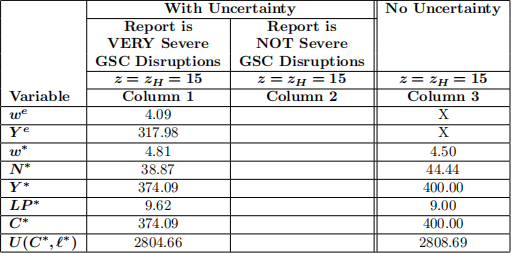
(1.B.) (9 points) Compare the level of household utility in Column 1 to the level of household utility in Column 3 and provide economic intuition for the direction of the difference between these two utility levels. Someone might argue that this result implies that households should ignore the announcement regarding GSC disruptions and always work 44.44 hours. Explain why they might argue this and explain why they are incorrect.

(1.C.) (10 points) For a general case in which the signal equals g and the productivity parameter equals zH, draw a single schematic PPF diagram to depict expected and equilibrium output, expected and equilibrium real wages, expected and equilibrium labour input, and the expected and equilibrium indifference curve of the household in the economy with uncertainty. On the same diagram, depict equilibrium output, real wages, labour input, and the indifference curve of the household in the economy without uncertainty.

You do not need to depict the household’s overall constraints. You do not need to draw the diagram for the specific example economy in this question – that turns out to be difficult because expected outcomes and equilibrium outcomes are fairly close together in the example and this makes it hard to draw both easily on the same diagram.

2. This question examines government spending financed by lump-sum taxes.

There is a single representative household which has h = 10 units of time which it can divide between working and leisure. The household’s preferences over consumption of the final good, leisure, and gov-ernment spending are given by the following utility function:

where λ is a constant to be specified below.

Production of the final good uses labour only with technology

where z fluctuates randomly between a relatively low level of and a relatively high level of 

The government finances government spending by lump-sum taxes equal to G = T imposed on the household. In periods in which productivity is high, the government does not spend or tax; G = T = 0. But in periods when productivity is low, the government may spend and tax at whatever level it takes to keep output at the same level as it is when productivity is high. That is, the government uses government spending and taxation to eliminate fluctuations in output.

(2.A.) (20 points) Complete Table 2.

Table 2: Lump-Sum Taxation

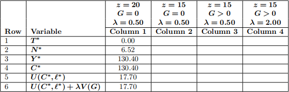
(2.B.) (11 points) Provide economic intuition for the direction of the change in each of the variables in Row 1-5 of Table 2 in moving from Column 2 to Column 3.

(2.C.) (8 points) Suppose λ = 2.00. From your results in Table 2, you should see that the household is better off when the government is following its policy of spending and taxing to maintain a constant level of output so one might conclude that stabilization policy is good for this economy. However, I would argue that the welfare gains that the household experiences under this stabilization policy do not really have anything to do with stabilizing output. Explain why I make that statement.

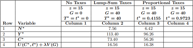
3. This question compares lump-sum taxes to proportional income taxes for financing government spending in our static model without capital.

Assume there is a representative household described exactly as in Question 2 with λ = 0.50. Assume there is a technology for final goods production described exactly as in Question 2.

There is a government who may spend G = 40 when The government may finance this by a lump-sum tax, T* = 40 or by a proportional income tax of the household. If the government uses a proportional income tax, according to my calculations, the government can finance this level of spending by imposing a tax at rate t* = 0.4155 or by imposing a tax at rate t* = 0.9723. That is for either rate, t*w*N* = 40 = G.

(3.A.) (18 points) Complete Table 3. Use economic intuition to explain the difference in the direction of change in labour input, N*, moving from Column 1 to Column 2 compared to moving from Column 1 to Column 3.

(3.B.) (9 points) Using your results from Table 3, rank the three different methods of taxation from best to worse if the government’s objective is to maximize household utility. Provide economic intuition for their ranking.

Table 3: Lump-Sum and Proportional Income Taxation