Programming Assignment CS4001/4042: Neural Networks and Deep Learning 2024

●    This assignment is to be done individually. You can discuss the questions with others but your submission must be your own unique work.

●    Data  files  and  other supporting  code for  both  parts are found  in the folder ‘Programming Assignment’ under ‘Assignments’ on NTULearn. You should use the  helper  codes  to  begin  and  provide  answers  to  the  assignment.  Please follow the formats given in helper codes to fill in your solutions. Those who do not   follow  the   specified  format  for  the   answers   risk   losing   marks   for presentation.

●    The assessment will be based on the correctness of the codes and solutions. Each part carries 45 marks, and 10 marks are assigned to the presentation and clarity of the solutions. The total number of marks is 100.

●    You  do   not  need  GPUs  for  this   assignment.   Local  PCs  will   be  sufficient. Attempt your assignments using Jupyter Lab / Notebook with version 3 and greater.

●    TAs  Mr.  Feng   Ruicheng  (RUICHENG002@e.ntu.edu.sg  ),  Ms.  Liang  Zhenxin ([email protected] ), and Mr. Liao Chang ([email protected]tu.edu.sg ) are in charge of this assignment.

●    For   any  inquiries,   please  either  contact  TAs   listed  above  or   post  in  the Discussion Board of NTULearn.

Submission procedure

●    Complete both parts A and B of the assignment and submit your solutions online via NTULearn before the deadline.

●    All submissions should be within the notebooks provided. Do not include data  nor model checkpoints in your submission. Submit 8 notebooks in this format:

o  For part A

.     <lastname>_<firstname>_Part_A_1.ipynb .     <lastname>_<firstname>_Part_A_2.ipynb .     <lastname>_<firstname>_Part_A_3.ipynb .     <lastname>_<firstname>_Part_A_4.ipynb .     common_utils.py

o  For Part B

.     <lastname>_<firstname>_Part  B  1.ipynb .     <lastname>_<firstname>_Part  B  2.ipynb .     <lastname>_<firstname>_Part  B  3.ipynb .     <lastname>_<firstname>_Part  B  4.ipynb

●    Late submissions will be penalized: 5% for each day up to three days.

Part A: Classification Problem

Part A of this assignment aims at  building  neural  networks to  perform  polarity detection from voice recordings, based on data in the National Speech Corpus, which is obtained from https://www.imda.gov.sg/how-we-can-help/national-speech-corpus

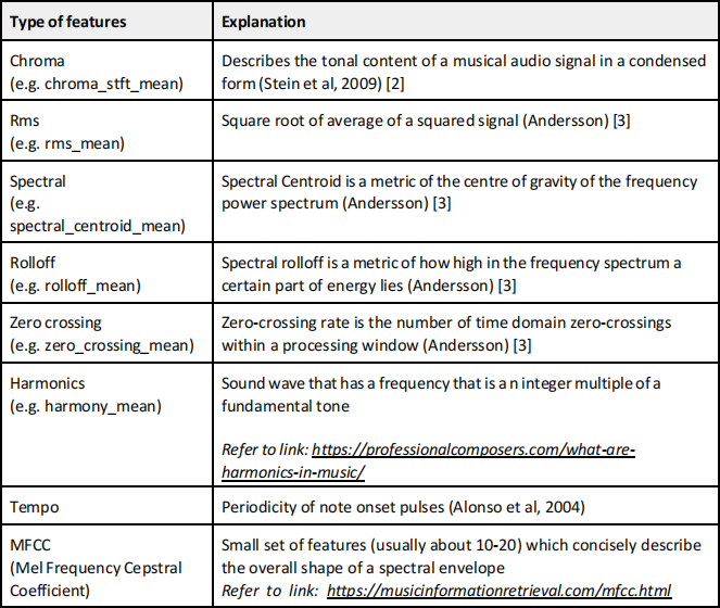
The   National  Speech  Corpus  is  an  initiative   by  the   Info-Communications  and   Media Development Authority, and it is the first large scale Singapore English corpus. Within the dataset, there  are  6  parts.  In  the  fifth  segment,  speakers  are  made  to  communicate  in several  different  styles,  including  Positive  Emotions  and  Negative  Emotions.  The  original recordings are approximately 20 minutes long. Using the librosa library, the recordings are split  into  shorter  segments  and  preprocessed  to   features  such  as  chromagrams,  Mel spectrograms, MFCCs and various other features.

The preprocessed CSV file is provided in this assignment. We will be using the CSV file named simplified.csv, which is both provided to you. The features from the dataset are engineered. The aim is to determine the speech polarity of the engineered feature dataset. The csv file is called simplified.csv with a row of 77 features that you can use, together with the filename. The “filename” column has the labels associated with them.

Question A1 (15 marks)

Design a feedforward deep neural network (DNN) which consists of three hidden layers of 128 neurons each with ReLU activation function, and an output layer with sigmoid activation function. Apply dropout of probability 0.2 to each of the hidden layers.

Divide the dataset into a 75:25 ratio for training and testing. Use appropriate scaling of input features. We solely assume that there are only two datasets here: training and test.

Use the training dataset to train the model for 100 epochs. Use a mini-batch gradient descent with ‘Adam’ optimizer with learning rate of 0.001, and batch size = 128. Implement early stopping with patience of 3.

Plot train and test accuracies and losses on training and test data against training epochs and comment on the line plots.

Question A2 (10 marks)

In this question, we will determine the optimal batch size for mini-batch gradient descent. Find the  optimal  batch  size  for  mini-batch  gradient  descent  by  training  the  neural  network  and evaluating the performances for different batch sizes. Note: Use 5-fold cross-validation on the training partition to perform hyperparameter selection. You will have to reconsider the scaling of the dataset during the 5-fold cross validation.

Plot mean cross-validation accuracies on the final epoch for different batch sizes as a scatter plot. Limit search space to batch sizes {64, 128, 256, 512, 1024}.

Next, create a table of time taken to train the network on the last epoch against different batch sizes.

Finally, select the optimal batch size and state a reason for your selection.

Question A3 (10 marks)

Find the optimal number of hidden neurons for the first depth and widths of the neural network designed in Question 1 and 2.

Plot the mean cross-validation accuracies on the final epoch for different combinations of depth and widths using a scatter plot. Limit the search space of the combos to {[64], [128], [256], [64, 64], [128, 128], [256, 256], [64, 128], [128, 64], [128, 256], [64, 256], [256, 128], [256, 64], [64, 64, 64], [128, 128, 128], [256, 256, 256], [64, 128, 256], [64, 256, 256], [128, 64, 64], [128, 128, 64], [256, 128, 64], [256, 256, 128]}. Continue using 5-fold cross validation on the training dataset.

Select the optimal combination for the depth and widths. State the rationale for your selection.

Plot the train and test accuracies against training epochs with the optimal combination of the depth and widths using   a  line plot.

[optional + 2 marks] Implement an alternative approach that searches through these combinations that could significantly reduce the computational time but achieve similar search results, without enumeration all the possibilities.

Note: use this optimal combination for the rest of the experiments.

Question A4 (10 marks)

In this section, we will explore the utility of such a neural network in real world scenarios.

Please use the real record data named ‘record.wav’  as a test sample. Preprocess the data using the provided preprocessing script (data_preprocess.ipynb) and prepare the dataset.

Do a model prediction on the sample test dataset and obtain the predicted label using a threshold of 0.5. The model used is the optimized pretrained model using the selected optimal batch size and optimal number of neurons.

Find the most important features on the model prediction for the test sample using SHAP. Plot the local  feature   importance  with   a  force   plot   and   explain   your   observations.   (Refer   to   the

documentation and these three useful references:

https://christophm.github.io/interpretable-ml-book/shap.html#examples-5,

https://towardsdatascience.com/deep-learning-model-interpretation-using-shap-a21786e91d16, https://medium.com/mlearning-ai/shap-force-plots-for-classification-d30be430e195)

Part B: Regression Problem

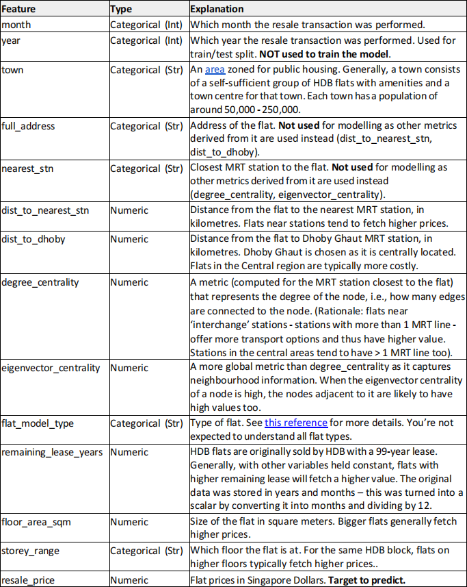
This assignment uses publicly available data on HDB flat prices in Singapore, obtained from data.gov.sg on  17th August 2023. The original dataset is combined with other datasets to include more informative features and they are given in the ‘hdb_price_prediction.csv’ file.

Question B1 (15 marks)

Real world  datasets  often  have  a  mix  of  numeric  and  categorical  features  –  this  dataset  is  one example. To build models on such data, categorical features have to be encoded or embedded.

PyTorch Tabular is a library that makes it very convenient to build neural networks for tabular data. It is built on top of PyTorch Lightning1, which abstracts away boilerplate model training code and makes it easy to integrate other tools, e.g. TensorBoard for experiment tracking.

For questions B1 and B2, the following features should be used:

- Numeric / Continuous features: dist  to   nearest_stn, dist  to  dhoby, degree_centrality, eigenvector_centrality, remaining_lease_years, floor_area_sqm

- Categorical features: month, town, flat_model_type, storey_range

Divide the dataset (‘hdb_price_prediction.csv’) into train, validation and test sets by using entries from year 2019 and before as training data, year 2020 as validation data and year 2021 as test data. Do not use data from year 2022 and year 2023.

Refer to the documentation of PyTorch Tabular and perform the following tasks: https://pytorch- tabular.readthedocs.io/en/latest/#usage

●    Use DataConfig to define the target variable, as well as the names of the continuous and categorical variables.

●    Use TrainerConfig to automatically tune the learning rate. Set batch_size to be 1024 and set max_epoch as 50.

●    Use CategoryEmbeddingModelConfig to create a feedforward neural network with 1 hidden layer containing 50 neurons.

●    Use OptimizerConfig to choose Adam optimiser. There is no need to set the learning rate (since it will be tuned automatically) nor scheduler.

●    Use TabularModel to initialise the model and put all the configs together.

Report the test RMSE error and the test R2  value that you obtained.

Printout the corresponding rows in the dataframe for the top 25 test samples with the largest errors. Identify a trend in these poor predictions and suggest a way to reduce these errors.

Question B2 (10 marks)

In Question B1, the default settings in PyTorch Tabular were enough to perform a quick experiment. In this part of the assignment, we will tryout a new model.

In  Question  B1,  we  used  the  Category   Embedding  model.  This  creates  a  feedforward  neural network in which the categorical features get learnable embeddings. In this question, we will make use of a library called Pytorch-WideDeep. This library makes it easy to work with multimodal deep- learning  problems combining  images, text, and tables. We will just  be  utilizing the deeptabular component of this library through the TabMlp network:

Divide the dataset (‘hdb_price_prediction.csv’) into train and test sets by using entries from the year 2020 and before as training data, and entries from 2021 and after as the test data.

Refer to the documentation of Pytorch-WideDeep and perform the following tasks:

https://pytorch-widedeep.readthedocs.io/en/latest/index.html

●    Use TabPreprocessor to create the deeptabular component using the continuous features and the categorical features. Use this component to transform the training dataset.

●   Create the TabMlp  model  with  2  linear  layers  in  the  MLP,  with  200  and  100  neurons respectively.

●   Create a Trainer for the training of the created TabMlp model with the root mean squared error (RMSE) cost function. Train the model for 100 epochs using this trainer, keeping a batch size of 64. (Note: set the num_workers parameter to 0.)

Report the test RMSE and the test R2 value that you obtained.

P.S. It is a good practice to try out standard machine learning models before using deep learning techniques. XGBoost is a popular option for tabular datasets.

Question B3 (10 marks)

Besides ensuring that your neural network performs well, it is important to be able to explain the model’s decision. Captum is a very handy library that helps you to do so for PyTorch models.

Many  model explainability algorithms for deep  learning  models  are  available  in Captum. These algorithms are often used to generate an attribution score for each feature. Features with larger scores are more ‘important’2   and some algorithms also provide information about directionality (i.e.  a feature with very negative attribution scores means the larger the value of that feature, the lower the value of the output).

In general, these algorithms can be grouped into two

paradigms:

-          perturbation based approaches (e.g. Feature Ablation)

-          gradient / backpropagation based approaches (e.g. Saliency)

The former adopts a brute-force approach of removing / permuting features one by one and does not scale up well. The latter depends on gradients and they can be computed relatively quickly. But unlike how backpropagation computes gradients with respect to weights, gradients here are computed with respect to the input. This gives us a sense of how much a change in the input affects the model’s outputs.

First, load the dataset following the splits in Question B1. To keep things simple, we will limit our analysis to numeric / continuous features only. Drop all categorical features from the dataframes. Do not standardise the numerical features for now.

Follow  this  tutorial  to   generate  the   plot  from  various   model   explainability  algorithms

(https://captum.ai/tutorials/House_Prices_Regression_Interpret).

Specifically, make the following changes:

- Use a feedforward neural network with 3 hidden layers, each having 5 neurons. Train using Adam optimiser with learning rate of 0.001.

- Use Saliency, Input x Gradients, Integrated Gradients, GradientSHAP, Feature Ablation

Train  a  separate  model  with  the   same  configuration  but  now  standardise  the  features  via StandardScaler  (fit  to  training  set,  then  transform  all).  State  your  observations  with  respect to GradientShap and explain why it has occurred.

(Hint: Many gradient-based approaches depend on a baseline, which is an important choice to be made. Check the default baseline settings carefully.)

Read https://distill.pub/2020/attribution-baselines/3 to build up your understanding of Integrated  Gradients (IG). You might find the following descriptions and comparisons in Captum useful as well.

Then, answer the following questions in the context of our dataset:

- Why did Saliency produce scores similar to IG?

- Why did Input x Gradients give the same attribution scores as IG?

Question B4 (10 marks)

Model degradation is a common issue faced when deploying machine learning models (including neural networks) in the real world. New data points could exhibit a different pattern from older data points due to factors such as changes in government policy or market sentiments. For instance, housing prices in Singapore have been increasing and the Singapore government has introduced 3 rounds of cooling measures over the past years (16 December 2021, 30 September 2022, 27 April 2023).

In  such  situations,  the  distribution  of  the  new  data  points  could  differ  from  the  original  data distribution which the models were trained on. Recall that machine learning models often work with the assumption that the test distribution should be similar to train distribution. When this assumption  is violated,  model  performance  will  be  adversely  impacted.  In  the  last  part  of  this assignment, we will investigate to what extent model degradation has occurred.

Your co-investigators used a linear regression model to rapidly test out several combinations of train/test splits and shared with you their findings in a brief report attached in Appendix A below. You wish to investigate whether your deep learning model corroborates with their findings.

Evaluate your model from B1 on data from year 2022 and report the test R2.

Evaluate your model from B1 on data from year 2023 and report the test R2.

Did model degradation occur for the deep learning model?

Model degradation could be caused by various data distribution shifts4 : covariate shift (features), label shift and/or concept drift (altered relationship between features and labels).

Using the Alibi Detect library, apply the TabularDrift function with the training data (year 2019 and before) used as the reference and detect which features have drifted in the 2023 test dataset. Before running the statistical tests, ensure you sample 1000 data points each from the train and test data.    Do    not    use    the    whole    train/test    data.     (Hint:    use    this    example    as    a   guide https://docs.seldon.io/projects/alibi-detect/en/stable/examples/cd_chi2ks_adult.html).

Assuming that the flurry of housing measures have made an impact on the relationship between all the features and resale_price (i.e. P(Y|X) changes), which type of data distribution shift possibly led to model degradation?

From your analysis via TabularDrift, which features contribute to this shift?

Suggest 1 way to address model degradation and implement it, showing improved test R2  for year 2023.

Appendix A

Here are our results from a linear regression model. We used StandardScaler for continuous variables and OneHotEncoder for categorical variables.

While 2021 data can be predicted well, test R2  dropped rapidly for 2022 and 2023.

Similarly, a model trained on 2017 data can predict 2018-2021 well (with slight degradation in performance for 2021), but drops drastically in 2022 and 2023.

With the test set fixed at year 2021, training on data from 2017-2020 still works well on the test data, with minimal degradation. Training sets closer to year 2021 generally do better.

References

[1] Koh JX, Mislan A, Khoo K, Ang B, Ang W, Ng C, Tan YY. Building the singapore english national speech corpus. Malay. 2019;20(25.0):19-3.
[2] Stein M, Schubert BM, Gruhne M, Gatzsche G, Mehnert M. Evaluation and comparison of audio chroma feature extraction methods. InAudio Engineering Society Convention 126 2009 May 1. Audio Engineering Society.
[3] Andersson T. Audio classification and content description. 2004.
[4] Miguel Alonso BD, Richard G. Tempo and beat estimation of musical signals. In
Proceedings of the International Conference on Music Information Retrieval (ISMIR), Barcelona, Spain 2004.