Lab 2 Instructions Microsoft Excel

Hello, dear friend, you can consult us at any time if you have any questions, add WeChat: daixieit

Lab 2 Instructions

Microsoft Excel

Lab Topic

Getting familiar with the spreadsheet working environment

Using formulas in Excel

Basic cell and data formatting in Excel

Background

In this lab, we will use the spreadsheet to calculate the future values of a periodical investment with a given interest rate. The formula used to calculate the investment’s value after n periods, the periodical interest rate r is:

In this formula:

· Pmt is the amount of investment in each period,

· r is the interest rate per period,

· n is the number of periods, and

· FV is the future value of the investment, i.e., how much money you will get after n periods.

Note r in this formula must be in a decimal format, e.g. 0.009 for 0.9% interest rate.

Practice

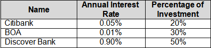
Assume that we want to divide our investment among three different organizations. The following table lists the composition and interest rate information.

Follow the procedures below to calculate the FV of our investments using Excel.

1. Download Lab 2 Investment Starter File.xlsx from Lab Assignments>>LA2 – Lab Assignment 2 in Blackboard.

2. Based on what you have learned in your lab sessions, you should know what are workbooks, worksheets, columns, rows, active cell, cell reference, etc.

3. Assume we plan to invest for 10 years, and each year, we plan to invest $12,000. Type these values in cells B4 and B6.

4. Format them as number and currency; number with 0 decimal places and currency with two.

5. We will use the annual interest rate to calculate the future value of our investment. Therefore, the number of periods should equal the number of years. Do not just type in this number in cell B5. Use the formula in cell B5 so that it’s equal to B4.

6. Enter the information for “annual interest rate” and “percentage of investment” from the shown above in the spreadsheet.

7. Calculate the investment amount for each bank per period in D10, D11, and D12. Use the product formula for multiplication.

8. In cell E10, type the formula “=(D10*(((1+B10)^B$5)-1))/B10” to calculate the FV of our investment in Citibank.

YOU MUST TYPE IN THIS FORMULA CAREFULLY AND CORRECTLY OR ELSE YOU WILL GET ERRORS.

Note the dollar sign “$” in the formula between “B” and “5”.

9. Move your mouse cursor over the lower-right corner of cell E10 until its shape changes into a cross. Hold down the mouse and drag it down to cell E12. Now check the formulas in E11 and E12; you’ll see that the dollar sign “$” keeps the reference cell number fixed.

10. Enter the totals in cells D15 and E15.

11. Answer the following questions using the worksheet.

a. Given the above portfolio, how many years do you need to invest to have at least

$1 million in your bank accounts? Type your answer next to the top highlighted cell which is L14.

Ø If the future values do not add up to over $1 million, adjust the “number of years” of your investment (B4) until it adds up.

Ø Then reset the value of B4 to “10”.

b. Following the same procedure, answer the question below:

Ø What’s the “amount per period” you must invest to have exactly $1 Million (up to 4 decimal places) in exactly 10 years?

12. Save your work in Excel format using this file naming convention:

LA02_Lastname_Firstname