PART 1 – SMOKING AND MORTALITY BIVARIATE REGRESSION

Hello, dear friend, you can consult us at any time if you have any questions, add WeChat: daixieit

PART 1 – SMOKING AND MORTALITY BIVARIATE REGRESSION

The purpose of this exercise is to help you learn the mechanics of ordinary least squares (OLS) regression and understand what the different terms in a regression mean. You will calculate the regression "by hand", and then you will use Excel to confirm the calculation.

Few medical professionals doubt that smoking leads to many health problems. While it is more difficult to determine that smoking raises the chance of death than simply to say that the two are positively related, in this assignment you will perform analysis that begins to document the relationship between smoking and mortality. However, this is far from a definitive analysis. The sample is very small, and no effort is made to control for other differences between the countries in the sample.

Historically, major factors contributing to excess mortality among smokers were thought to include respiratory disease, vascular disease, cancers, and others. We will label death from these diseases as smoking-related deaths.

Smoking-related deaths in 1950 and per capita cigarette consumption in 1930 are shown below for five countries. The smoking-related deaths are shown for a later time period because it presumably takes time for health problems to arise from smoking. Our hypothesis (obviously) is that the dependent variable, smoking-related deaths (Y), is a function of the independent variable, cigarette consumption (X).

1. What is the Population Regression Function (PRF) for the relationship between Smoking-Related Deaths per million people in 1950 and Cigarettes Consumed per capita in 1930?

To write out the equation, you can type using words (e.g. Beta_1 or Beta_1_Hat or Cigs_i) or Word’s equation functionality, or you could write the equation by hand and insert an image of it.

The figure below illustrates the data points for each country. The x-axis records our measure of cigarette consumption, and the y-axis records our measure of smoking-related deaths. The blue line is an illustration of the line of best fit in terms of least squares. The light blue and green lines with arrows record the change in the Y variable and the change in the X variable for each line segment.

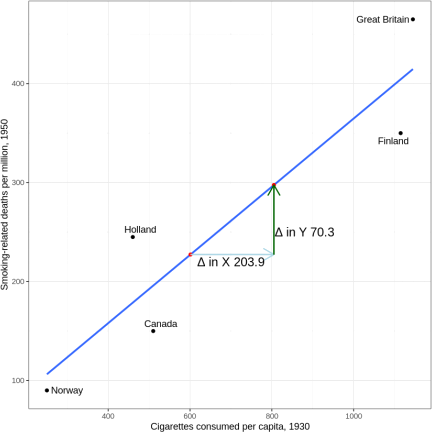
2. What is the Sample Regression Function (SRF) for the countries plotted above?

3. Show how to calculate each of the following quantities.

Though you will never do this in an actual analysis, we would like you to go through the exercise of manually constructing the quantities we estimated in the Sample Regression Function. Please compute the answer to each question, showing and/or explaining your work where relevant. For each, explain the substantive interpretation of what you calculated.

Hint: Note that the following formulas apply:

 (Change in Y divided by change in X)

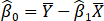 (Where  is the average value for Y, and the same for )

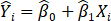 (The predicted value of Y for each country)

 (The residual for each country)

Note: You may use Excel to do the calculations as long as you do not use the built-in regression function. Alternatively, you can calculate them by hand.

Space for showing calculations:

a. , the estimated slope coefficient from the sample regression function.

b. , the estimated intercept term from the same regression.

c. , the predicted values for each country.

d. , the residuals/error terms for each country.

e. , the sum of squared residuals.

Note: You do not need to interpret this quantity. Unlike the other quantities you estimated, this number by itself does not tell us much. The calculations that you did above generated a line that minimizes this quantity.

4. In a concise paragraph drawing on the numbers you calculated above, describe the relationship between national smoking and smoking-related death rates as precisely as you can. Indicate the direction and magnitude of the relationship based on this sample.

Now you will estimate the same regression you ran before but this time in Excel.

You can familiarize yourself with running regressions in Excel by referring to section notes.

5. In Excel, using the data provided above, run a linear regression of smoking-related deaths per million (deaths) in cigarette consumption per capita (cigs). From the summary Excel output, find and label  and  (see class notes and TF session materials for guidance). Do the values for these estimates match the quantities you calculated above?

Please paste your regression results below, in addition to answering the questions.

6. Consider the hypothesis H0:  = 0 in the context of the above regression.

a. Why would you be interested in testing this hypothesis?

a. Would you reject the hypothesis H0:  = 0 at the 5% significance level? Explain.

PART 2 – POLITICAL PARTICIPATION

Congratulations! You've secured an internship with an organization headquartered in Massachusetts whose mission is to increase political participation and political engagement. They've been looking for a data analyst, and you have been selected to fill that role. The organization is particularly interested in learning more about how to engage with young voters (defined optimistically here as voters under the age of 30).

You will be gathering insights into people’s political behavior based on the Cooperative Congressional Election Study (CCES, https://doi.org/10.7910/DVN/E9N6PH). The CCES is an online survey that is conducted in the last quarter of every year. In election years, the survey is administered in two waves with a set of questions before the election and a set of questions after the election. The survey seeks to help researchers understand the political preferences and behaviors of American voters.

The CCES data you will be using contains individual-level survey responses for 2016 and 2020. Furthermore, the file has been matched to state voter files in order to confirm whether respondents turned out to vote in a given election year. The survey is based on an online panel conducted by a survey film called YouGov.

Let’s begin by opening the dataset in Excel and inspecting the variables.

The table below lists key variables contained in the CCES data. The Variable column denotes the name of the variable; the Description column provides a brief explanation of the variable; the Variable Type column denotes the type of variable. A numeric variable is one that is defined on the real number line. You can perform numeric operations (adding, subtracting, multiplying, dividing, etc.) on such variables. Factor variables are categorical. For example, the education level variable (educ) is categorical, with categories consisting of No HS, High School Graduate, 2-Year, Some College, 4-Year, and Post-Grad.

Campaign Donations

Campaign donations are a key form of political participation. The CCES asks respondents if they have donated and how much money they have donated to political campaigns in the past year.

The organization you work for is particularly interested in the questions: Who chooses to donate to a political campaign and who does not? Are older people more likely to donate more money than younger people? To study this question, we can use the variable total_donations. Your goal is to examine what variables have the strongest relationship with the amount donated to a political campaign.

1. Plot the relationship between Donations ($) and Age using a scatter plot where each point represents the average donation level among people of a certain age in 2020.

Hint 1: To create a dataset with binned donation averages by age, use a PivotTable where the Rows are “age” and the Values are the “Average” of total_donations.

Hint 2: To make a scatterplot based on a PivotTable, you may have to copy the PivotTable’s contents to a different set of columns and use the new columns to make your plot.

2. Divide the sample into people who are under the age of 30 (age<30) and people who are 30 and above (age≥30). What is the difference in average donations between people below 30 versus 30 and above? You do not need to evaluate the statistical significance of this difference.

Hint: Use the “=IF( )” code referenced in the class size example from class to help you make this new variable, and then use a PivotTable to see average values for each group.

3. Now regress total donations on a variable you create indicating respondents who are below age 30. Is your answer similar or different from the results from Question 2? Is the estimate of the coefficient statistically significant?

Please paste your regression results below, in addition to answering the questions.

4. Estimate a regression model where the outcome variable is the total amount donated (total_donations) and the explanatory variable is age (age). Then, describe: What is the association between age and the amount donated? Does this association surprise you, given the scatter plot that you made in response to a prior question? Is the association statistically significant?

Please paste your regression results below, in addition to answering the questions.

Age and Turnout

Now let’s examine the relationship between a state’s average age and average turnout for people between the ages of 18 and 85. First, we will collapse across respondents based on state and age to create a new state-level data set.

You can use the same procedure as above but this time, use both “year” and “st” as rows, and the average of “age” and “voted” as Values.

5. Create a single plot that illustrates the relationship between the average age of survey respondents in a state and the turnout rate for that state in 2016 and 2020. To be clear, this should be one plot that (1) distinguishes between the data for 2016 and 2020; (2) contains points that plot the average age and average turnout rate for each state in each year; and (3) allows the reader to see the statistical relationship between age and turnout for each year (i.e. fits a separate line to the data for each year).

Hint 1: You can then make a scatter plot that includes both sets of data, 2016 and 2020. The easiest way to do this is to create a blank scatterplot, right click on it and click “Select Data…”, then make two separate “Series,” one for 2016 and one for 2020.

Hint 2: You can add a trend line for each year using the “Add Chart Element” tab.

6. Estimate separate regression models for 2016 and 2020 of the relationship between state-level turnout and state-level average age. Interpret the coefficients. Is the coefficient for the relationship between turnout and age similar for each year? What about the intercept term?

Please paste your regression results below, in addition to answering the questions.