Stochastic Simulation Coursework 2023

1 Stochastic Simulation - Coursework 2023

This assignment has two parts and graded over 100 marks.  Some general remarks:

•  The assignment is due on 11 December 2023, 1PM GMT, to be submitted via Blackboard (see the instructions on the course website).

•  You should use this .ipynb file as a skeleton and you should submit a PDF report.  Prepare the IPython notebook and export it as a PDF. If you can’t export your notebook as PDF, then you can export it as HTML and then use the “Print” feature in browser (Chrome: File -> Print) and choose “Save as PDF”.

•  Your PDF should be no longer than 20 pages. But please be concise.

•  You can reuse the code from the course material but note that this coursework also requires novel implementations. Try to personalise your code in order to avoid having problems with plagiarism checks. You can use Python’s functions for sampling  random variables of all distributions of your choice.

• Please comment your code properly.

Let us start our code.

[ ]: import matplotlib.pyplot as plt

import numpy as np

rng = np.random.default_rng(36) # You can change this.

1.1 Q1: Model Selection via Perfect Monte Carlo (40 marks)

Consider the following probabilistic model

p(x) = N(x; 5, 0.01),

p(gi |x) = N(gi ; θx, 0.05),

for i = 1, … , T where gi  are conditionally independent given 从.  You are given a dataset (see it on Blackboard) denoted here as g1∶T  for T = 100.  As defined in the course, we can find the marginal likelihood as

pθ (g1∶T ) = ∫ pθ (g1∶T |从)p(从)d从,

where we have left θ-dependence in the notation to emphasise that the marginal likelihood is a function of θ .

Given the samples from prior p(x), we can identify our test function above as Ψ(x) = pθ (g1∶T |x).

(i) The first step is to write a log-likelihood function of g1∶T , i.e., pθ (g1∶T |x).  Note that, this is the joint likelihood of conditionally i.i.d.  observations gi  given x.  This function should take input the data set vector y as loaded from y_perfect_mc.txt below,  θ (scalar),  and  x (scalar),  and sig (likelihood variance which is given as 0.05 in the question but leave it as a variable) values to evaluate the log-likelihood.  Note that log-likelihood will be a sum in this case, over individual log-likelihoods. (10 marks)

[ ]: # put the dataset in the same folder as this notebook

# the following line loads y_perfect_mc.txt

y = np.loadtxt('y_perfect_mc.txt')

y = np.array(y, dtype=np.float64)

# fill in your function below.

def log_likelihood(y, x, theta, sig): # fill in the arguments

# fill in the function

pass # remove this line

return # fill in the return value

# uncomment and evaluate your likelihood (do not remove)

# print(log_likelihood(y, 1, 1, 1))

# print(log_likelihood(y, 1, 1, 0.1))

# print(log_likelihood(y, -1, 2, 0.5))

(ii) Write a logsumexp function. Let v be a vector of log-quantities and assume we need to compute log ∑ 1 exp(vi ) where v = (v1 , … , vN ).  This function is given as

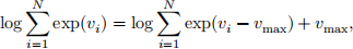
where vmax  = maxi=1,…,N vi .  Implement this as a function which takes a vector of log-values and returns the log of the sum of exponentials of the input values. (10 marks)

[ ]: def logsumexp(v):

# v is a vector

# fill in the function

pass # remove this line

# uncomment and evaluate your logsumexp function (do not remove)

# print(logsumexp(np.array([1, 2, 3])))

# print(logsumexp(np.array([1, 2, 3, 4, 5, 6, 7, 8, 9, 10])))

# print(logsumexp(np.array([5, 6, 9, 12])))

(iii) Now we are at the stage of implementing the log marginal likelihood estimator.  Inspect your estimator as described in Part (i).  Its particular form is not implementable without using the trick you have coded in Part (iii). Now, implement a function that returns the log of the MC estimator you derived in Part (i). This function will take in

•  y dataset vector

•  θ parameter (scalar)

•  x_samples (np.array vector) which are N Monte Carlo samples.

•  a variance  (scalar) variable  sig for the joint log likelihood pθ (g1∶T |x) that will be used in log_likelihood function (we will set this to 0.05 as given in the question).

Hint: Notice that the log of the MC estimator of the marginal likelihood takes the form

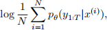
as given in the question.  You have to use pθ (g1∶T |x(i)) = exp(log pθ (g1∶T |x(i))) to get a logsumexp structure, i.e., log and sum (over particles) and exp of log pθ (g1∶T |x(i)) where i = 1, … , N and x(i) are the N Monte Carlo samples (do not forget 1/N term too). Therefore, now use the function of Part (i) to compute log pθ (g1∶T |x(i)) for every i = 1, … , N and Part (ii) logsumexp these values to compute the estimate of log marginal likelihood. (10 marks)

[ ]: def log_marginal_likelihood(y, theta, x_samples, sig): # fill in the arguments

# fill in the function

pass # remove this line

return # fill in the return value

# uncomment and evaluate your marginal likelihood (do not remove)

# print(log_marginal_likelihood(y, 1, np.array([-1, 1]), 1))

# print(log_marginal_likelihood(y, 1, np.array([-1, 1]), 0.1))

# print(log_marginal_likelihood(y, 2, np.array([-1, 1]), 0.5))

# note that the above test code takes 2 dimensional array instead of N␣ ↪particles for simplicity

(iv) We will now try to find the most likely θ . For this part, you will run your log_marginal_likelihood function for a range of θ values. Note that,  for every  θ value,  you need to sample N new samples from the prior  (do not reuse the same samples).  Compute your estimator of the log M(N)C  ≈ log pθ (g1∶T) for θ-range given below.  Plot the log marginal likelihood estimator as a function of θ . (5 marks)

[ ]: sig = 0.05

sig_prior = 0.01

mu_prior = 5.0

N = 1000

theta_range = np .linspace(0, 10, 500)

log_ml_list = np .array([]) # you can use np.append to add elements to this array

# fill in your code here

# uncomment and plot your results (do not remove)

# plt.plot(theta_range, log_ml_list)

# plt.x label(r'$\theta$')

# plt.y label(r'$\log p_\theta(y_{1:T})$')

# plt.show()

(v) Now  you  have   log_ml_list variable  that   corresponds  to   marginal  likelihood  values   in theta_range.   Find the θ value that gives the maximum value in this list and provide your fi- nal estimate of most likely θ . (5 marks)

[ ]: # You code goes here

# print your theta estimate, e.g.:

# print(theta_est)

1.2 Q2: Posterior sampling (35 marks)

In this question, we will perform posterior sampling for the following model

p(x) ∝ exp(−x1(2)/10 − x2(2)/10 − 2(x2  − x1(2))2 ),

p(g|x) = N(g; Hx, 0.1)

where H =  [0, 1].   In this exercise,  we assume that we have observed g = 2 and would like to implement a few sampling methods.

Before starting this exercise, please try to understand how the posterior density should look like. The discussion we had during the lecture about Exercise 6.2 (see Panopto if you have not attended) should help you here to understand the posterior density. Note though quantities and various details are different here.  You should have a good idea about the posterior density before starting this exercise to be able to set the hyperparameters such as the chain-length, proposal noise, and the step-size.

[ ]: y = np.array([2.0])

sig_lik = 0.1

H = np.array([0, 1])

(i) In what follows, you will have to code the log-prior and log-likelihood functions.  Do not use any library, code the log densities directly. (5 marks)

[ ]: def prior(): # code banana density for visualisation purposes

# fill in the function

pass # remove this line

return # fill in the return value

def log_prior(): # fill in the arguments

# fill in the function

pass # remove this line

return # fill in the return value

def log_likelihood(): # fill in the arguments

# fill in the function

pass # remove this line

return # fill in the return value

# uncomment below and evaluate your prior and likelihood (do not remove)

# print(log_prior([0, 1]))

# print(log_likelihood(y, np.array([0, 1]), sig_lik))

(ii) Next, implement the random walk Metropolis algorithm (RWMH) for this target.  Set an appropriate chain length, proposal variance, and burnin value.  Plot a scatter-plot with your samples (see the visualisation function below). Use log-densities only. (10 marks)

[ ]: # fill in your code here

# uncomment and plot your results (do not remove)

# x_bb = np.linspace(-4, 4, 100)

# y_bb = np.linspace(-2, 6, 100)

# X_bb , Y_bb = np.meshgrid(x_bb , y_bb)

# Z_bb = np.zeros((100 , 100))

# for i in range(100):

#     for j in range(100):

#         Z_bb[i, j] = prior([X_bb[i, j], Y_bb[i, j]])

# plt.contourf(X_bb , Y_bb , Z_bb , 100 , cmap='RdBu')

# plt.scatter(x[:, 0], x[:, 1], s=10 , c='white')

# plt.show()

# Note that above x vector (your samples) is assumed to be (N, 2).

# It does not have to be this way (You can change the name of the variable x␣ ↪ too).

# i.e., If your x vector is (2, N), then use

# plt.scatter(x[0, :], x[1, :], s=10 , c='white')

# instead of

# plt.scatter(x[:, 0], x[:, 1], s=10 , c='white')

# in the above code.

(iii) Now implement Metropolis-adjusted Langevin algorithm.   For this,  you will need to code the gradient of the density and use it in the proposal as described in the lecture notes.  Set an appropriate chain length, step-size, and burnin value.  Plot a scatter-plot with your samples (see the visualisation function below). Use log-densities only. (10 marks)

[ ]: def grad_log_prior(): # fill in the arguments

# fill in the function

pass # remove this line

return # fill in the return value

def grad_log_likelihood(): # fill in the arguments

# fill in the function

pass # remove this line

return # fill in the return value

def log_MALA_kernel(): # fill in the arguments

# fill in the function

pass # remove this line

return # fill in the return value

gam = 0.01

# fill in your code here

# uncomment and plot your results (do not remove)

# x_bb = np.linspace(-4, 4, 100)

# y_bb = np.linspace(-2, 6, 100)

# X_bb , Y_bb = np.meshgrid(x_bb , y_bb)

# Z_bb = np.zeros((100 , 100))

# for i in range(100):

#     for j in range(100):

#         Z_bb[i, j] = prior([X_bb[i, j], Y_bb[i, j]])

# plt.contourf(X_bb , Y_bb , Z_bb , 100 , cmap='RdBu')

# plt.scatter(x[:, 0], x[:, 1], s=10 , c='white')

# plt.show()

# Note that above x vector (your samples) is assumed to be (N, 2).

# It does not have to be this way (You can change the name of the variable x␣ ↪ too).

# i.e., If your x vector is (2, N), then use

# plt.scatter(x[0, :], x[1, :], s=10 , c='white')

# instead of

# plt.scatter(x[:, 0], x[:, 1], s=10 , c='white')

# in the above code.

(iv) Next,  implement unadjusted Langevin algorithm.   For this, you will need to code the gradient of the density and use it in the proposal as described in the lecture notes.  Set an appro- priate chain length, step-size, and burnin value.  Plot a scatter-plot with your samples  (see the visualisation function below). Use log-densities only. (10 marks)

[ ]: # fill in your code here

# uncomment and plot your results (do not remove)

# x_bb = np.linspace(-4, 4, 100)

# y_bb = np.linspace(-2, 6, 100)

# X_bb , Y_bb = np.meshgrid(x_bb , y_bb)

# Z_bb = np.zeros((100 , 100))

# for i in range(100):