Problem Set 5

Hello, dear friend, you can consult us at any time if you have any questions, add WeChat: daixieit

Problem Set 5

This is the final homework assignment, which accounts for 35% of your final grade. Unlike the previous problem sets, you are required to collect the data on your own and conduct data analysis based on your collected data.

If you decide not to submit the problem set 4, the weight of the problem set 5 will increase from 35% to 50%.

You may work with other students. The maximum number of students per group is two. However, you can work on your own. Be sure to indicate with whom you have worked in your submission.

Deadline: Dec 15, 2023 (HK Time 5 PM).

There is a penalty for late submissions: 5% will be subtracted from the total mark for every additional day after the deadline. If you submit it after Dec 25, 2023, you will get a zero on this homework assignment.

WRDS course account:

Account name: mfin7033_2023

Password: girjYt-vajtic-tygbu2

Reference

Ang, A., Hodrick, R. J., Xing, Y., & Zhang, X. (2006). The cross-section of volatility and expected returns. Journal of Finance, 61(1), 259-299.

Background

In this problem set, you will examine the pricing of aggregate and idiosyncratic volatility risk in the cross-section of stock returns, following the Journal of Finance paper Ang, Hodrick, Xing, and Zhang (2006) (thereafter, AHXZ (2006)). Specifically, we ask the following questions: Do the stocks with larger exposures to the volatility risk earn higher or low average returns?

To answer this question, we need first to find a measure of the volatility exposure. Following AHXZ (2006), we consider the VIX index. The VIX index is constructed so that it represents the implied volatility of a synthetic at-the-money option contract on the S&P100 index that has a maturity of 1 month. It is constructed from eight S&P100 index puts and calls and takes into account the American features of the option contracts, discrete cash dividends, and microstructure frictions such as bid– ask spreads.

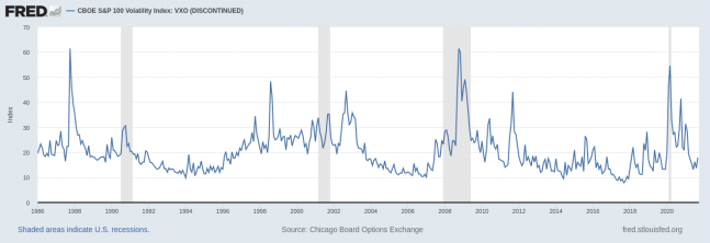
Because the VIX index is highly serially correlated with a first-order autocorrelation of 0.94, we measure daily innovations in aggregate volatility by using daily changes in VIX, which we denote as ΔVIX.

There are four parts in this problem set.

Part I. Main Findings of AHXZ (2006)

In this part, you need to summarise the main findings in AHXZ (2006). Please list the two findings that you think are the most important (there are more than two, but you do not have to list all of them). For each key finding, please provide an economic explanation of the empirical phenomenon.

Part II. Collecting Data

The monthly and daily individual stock data come from CRSP, accounting data come from COMPUSTAT, and data on the CBOE implied volatility index, VIX, come from the FRED st louis. To be clear, AHXZ (2006) use the SP100-based implied volatility index, which has a ticker of VXO, for all tests reported in this paper. You can further download the Fama-French three factors (market, size, and value factors) from Ken French's website. I provide some useful links to several datasets at the end of this document.

Your first task is to download all the data and load the datasets using pandas . After that, you need to report (1) which datasets you use in this problem set and why you need them, (2) how you preprocess the data (e.g., dropping samples based on some requirements, handling missing data, merging datasets, etc.), and (3) how many firms per year your final sample has in the panel data of stock returns.

Part III. Pricing Aggregate Volatility Shocks

To measure the sensitivity to aggregate volatility innovations, you are required to run the following regression:

where:

MKT is the daily market excess return,

ΔVIXt is the daily change in the VIX index, and

βiMKT and βiΔVIX are firm i's loadings on market risk and aggregate volatility risk, respectively.

You need to run the regression ( ) with daily data for each stock per month. Specifically, for each month, you run the regression for all stocks on AMEX, NASDAQ, and the NYSE, with more than 17 daily observations and obtain the monthly estimates of βiMKT and βiΔVIX. In this step, you will need to use the CRSP daily stock return data and also the market and VIX daily data. When you estimate the regression ( ) with daily data, please ignore the delisting returns. It does not mean that the delisting returns are not important; instead, handling delisting returns at daily frequency is too involving and out of the scope of this course.

At the end of each month, you sort stocks into quintiles based on the value of the realized coefficients over the past month. Firms in quintile 1 have the lowest coefficients, while firms in quintile 5 have the highest loadings. Within each quintile portfolio, we value-weight the stocks. We link the returns across time to form one series of post-ranking returns for each quintile portfolio. In this portfolio sorting step, you should use the CRSP monthly stock return data. At the monthly frequency, you should consider the delisting returns.

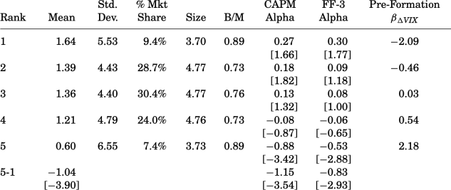
Your task is to replicate the empirical results in Table I of AHXZ (2006). Please only replicate the numbers in the following attached table.

The first two columns report the mean and standard deviation of the monthly total, not excess, simple returns.

The column labelled % Mkt share shows the percentage of market cap for all the stocks in each quintile.

The columns labelled size and B/M show the average log market capitalization and book-to-market ratio for firms within the portfolio (You do NOT need to replicate these two columns).

The columns labelled “CAPM Alpha” and “FF-3 Alpha” report the time-series alphas of these portfolios relative to the CAPM and to the FF-3 model, respectively.

The final column reports the pre-formation βiΔVIX coefficients, which are computed at the beginning of each month for each portfolio and are value-weighted.

Part IV. Pricing Idiosyncratic Volatility

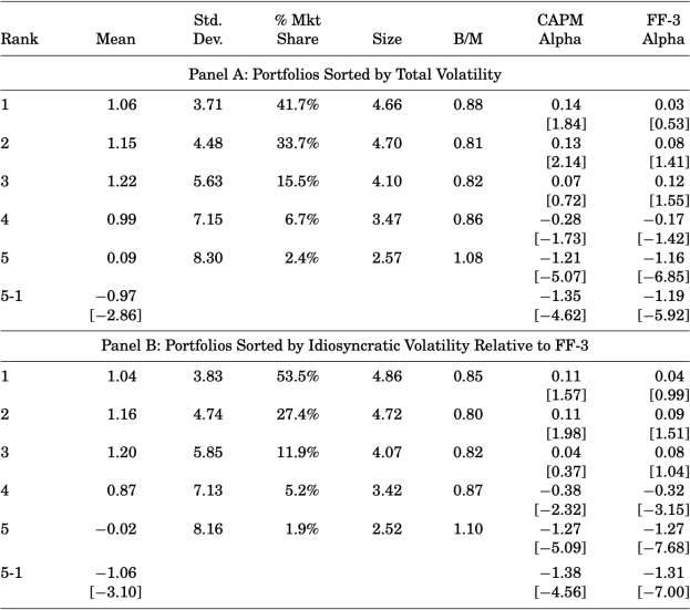
In this section, we investigate a second set of assets sorted by idiosyncratic volatility defined relative to the FF-3 model. If market volatility risk is a missing component of systematic risk, standard models of systematic risk, such as the CAPM or the FF-3 model, should misprice portfolios sorted by idiosyncratic volatility because these models do not include factor loadings measuring exposure to market volatility risk.

We estimate the idiosyncratic volatility as follows (Use the daily observations per month to estimate the following regression, with more than 17 daily observations):

Next, idiosyncratic risk is defined as in equation ( ). Finally, we sort the stocks into quintile portfolios based on idiosyncratic volatility ( ). You need to replicate Table VI (Panel B only) of AHXZ (2006), as shown below:

The sample period in AHXZ (2006) is from January 1986 to December 2000. You need to repeat the above analysis for three sample periods (in both Part III and IV):

January 1986 to December 2000,

January 2001 to December 2020, and

January 1986 to December 2020.

Does the long-short portfolio (marked as 5-1 above) have stable performance over different subsamples? How do you interpret your findings?

Caveat: It is impossible to get exactly the same numbers as in the original paper.

Some useful links:

VXO/VIX index: https://wrds-www.wharton.upenn.edu/pages/get-data/cboe-indexes/cboe-indexes-1/cboe-indexes/ or https://fred.stlouisfed.org/series/VXOCLS

Ken French's library: https://mba.tuck.dartmouth.edu/pages/faculty/ken.french/data_library.html

CRSP Stock / Security Files: https://wrds-www.wharton.upenn.edu/pages/get-data/center-research-security-prices-crsp/annual-update/stock-security-files/

Compustat: https://wrds-www.wharton.upenn.edu/pages/get-data/compustat-capital-iq-standard-poors/compustat/north-america-daily/

Submission Requirement

You need to submit two documents:

A PDF file that contains your explanation of the above four parts, such as the main findings, economic explanations, execution details, etc.

Python codes (Jupyter Notebook, .py file, etc.) that show the details in your data work.

Your grade is determined by the accuracy of your solutions, explanations of each data analysis step, and your interpretation of the empirical findings.

Please do not submit the datasets onto Moodle. Instead, you can create a Dropbox (or Google Drive or Microsoft OneDrive) link to share the datasets with me. Alternatively, you can use SQL (see lecture 11) to select the data. If you go in this way, you do not need to create the Dropbox or Google Drive link but show the SQL commands as follows:

##############

# CRSP Block #

##############

# a.permno: unique permanent security identification number assigned by CRSP to each security;

# a.permco: CRSP Permanent Company Number;

# b.shrcd: Share Code, common equity has shrcd 10 or 11;

# b.exchcd: Exchange Code, 1 is NYSE, 2 is AMEX and 3 is NASDAQ;

# a.ret: Holding Period Return;

# a.retx: Holding Period Return without Dividends;

# a.shrout: Number of Shares Outstanding;

# a.prc: Price

# Get monthly stock data from "crsp.msf" (CRSP Monthly Stock):

crsp_m = conn.raw_sql("""

SELECT a.permno, a.permco, a.date, b.shrcd, b.exchcd,

a.ret, a.retx, a.shrout, a.prc, b.siccd

FROM crsp.msf as a

LEFT JOIN crsp.msenames as b

ON a.permno=b.permno

AND b.namedt<=a.date

AND a.date<=b.nameendt

WHERE a.date between '01/01/1960' and '12/31/2022'

AND b.exchcd between 1 and 3

""")

Finally, if you find anything unclear, please read the JF paper, AHXZ (2006), carefully.