关键词 > Python代写
Artificial Intelligence in Games Assignment 2
发布时间:2023-12-16
Hello, dear friend, you can consult us at any time if you have any questions, add WeChat: daixieit
Assignment 2
Artificial Intelligence in Games
In this assignment, you will implement a variety of reinforcement learning algorithms to find policies for the frozen lake environment. Please read this entire document before you start working on the assignment.
The code presented in this section uses the NumPy library. If you are not familiar with NumPy, please read the NumPy quickstart tutorial and the NumPy broadcasting tutorial.
The frozen lake environment has two main variants: the small frozen lake (Fig. 1) and the big frozen lake (Fig. 2). In both cases, each tile in a square grid corresponds to a state. There is also an additional absorbing state, which will be introduced soon. There are four types of tiles: start (grey), frozen lake (light blue), hole (dark blue), and goal (white). The agent has four actions, which correspond to moving one tile up, left, down, or right. However, with probability 0.1, the environment ignores the desired direction and the agent slips (moves one tile in a random direction, which may be the desired direction). An action that would cause the agent to move outside the grid leaves the state unchanged.
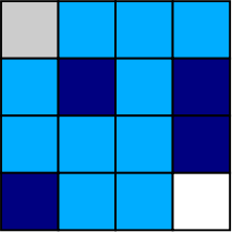
Figure 1: Small frozen lake
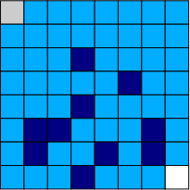
Figure 2: Big frozen lake
The agent receives reward 1 upon taking an action at the goal. In every other case, the agent receives zero reward. Note that the agent does not receive a reward upon moving into the goal (nor a negative reward upon moving into a hole). Upon taking an action at the goal or in a hole, the agent moves into the absorbing state. Every action taken at the absorbing state leads to the absorbing state, which also does not provide rewards. Assume a discount factor of γ = 0.9.
For the purposes of model-free reinforcement learning (or interactive testing), the agent is able to interact with the frozen lake for a number of time steps that is equal to the number of tiles.
Your first task is to implement the frozen lake environment. Using Python, try to mimic the interface presented in Listing 1.
Listing 1: Frozen lake environment.
import numpy as np
import contextlib
# Configures numpy print options
@contextlib . contextmanager
def printoptions (* args , ** kwargs ) :
original = np . get ![]() printoptions ()
printoptions ()
np . set printoptions (* args , ** kwargs )
try :
yield
finally :
np . set printoptions (* * original )
class EnvironmentModel :
def in it ( self , n states , n actions , seed=None ) :
self . n states = n states
self . n actions = n actions
self . random ![]() state = np . random . RandomState( seed )
state = np . random . RandomState( seed )
def p( self , next state , state , action ) :
raise NotImplementedError ()
def r ( self , next state , state , action ) :
raise NotImplementedError ()
def draw( self , state , action ) :
p = [ self . p( ns , state , action ) for ns in range( self . n ![]() states ) ]
states ) ]
next ![]() state = self . random
state = self . random ![]() state . choice ( self . n
state . choice ( self . n ![]() states , p=p)
states , p=p)
reward = self . r ( next ![]() state , state , action )
state , state , action )
return next state , reward
class Environment ( EnvironmentModel ) :
def in it ( self , n states , n actions , max steps , pi , seed=None ) :
EnvironmentModel . in it ( self , n ![]() states , n
states , n ![]() actions , seed )
actions , seed )
self . max steps = max steps
self . pi = pi
if self . pi is None :
self . pi = np . full ( n ![]() states , 1./ n
states , 1./ n ![]() states )
states )
def reset ( self ) :
self . n steps = 0
self . state = self . random ![]() state . choice ( self . n
state . choice ( self . n ![]() states , p=self . pi )
states , p=self . pi )
return self . state
def step ( self , action ) :
if action < 0 or action >= self . n actions :
raise Exception ( ’ Invalid ![]()
![]() action . ’ )
action . ’ )
self . n steps += 1
done = ( self . n ![]() steps >= self . max
steps >= self . max ![]() steps )
steps )
self . state , reward = self . draw( self . state , action )
return self . state , reward , done
def render ( self , policy=None , value=None ) :
raise NotImplementedError ()
class FrozenLake ( Environment ) :
def ” ” ![]() n it
n it ( self , lake , slip , max steps , seed=None ) :
lake : A matrix that represents the lake . For example :
lake = [[ ’& ’ , ’. ’ , ’. ’ , ’. ’] ,
[ ’. ’ , ’#’, ’. ’ , ’# ’] ,
[ ’. ’ , ’. ’ , ’. ’ , ’# ’] ,
[ ’# ’ , ’. ’ , ’. ’ , ’$ ’] ]
slip : The probability that the agent will slip
max steps : The maximum number of time steps in an episode
seed : A seed to control the random number generator ( optional )
”””
# start (&) , frozen (.) , hole (#), goal ($)
self . lake = np . array ( lake )
self . lake ![]() flat = self . lake . reshape (−1)
flat = self . lake . reshape (−1)
self . slip = slip
n states = self . lake . size + 1
n actions = 4
pi = np . zeros ( n ![]() states , dtype=float )
states , dtype=float )
pi [ np . where ( self . lake flat == ’&’ ) [ 0 ] ] = 1.0
self . absorbing state = n states − 1
# TODO:
Environment . in it ( self , n ![]() states , n
states , n ![]() actions , max steps , pi , seed=seed )
actions , max steps , pi , seed=seed )![]()
def step ( self , action ) :
state , reward , done = Environment . step ( self , action )
done = ( state == self . absorbing ![]() state ) or done
state ) or done
return state , reward , done
def p( self , next state , state , action ) :
# TODO:
def r ( self , next state , state , action ) :
# TODO:
def render ( self , policy=None , value=None ) :
if policy is None :
lake = np . array ( self . lake ![]() flat )
flat )
if self . state < self . absorbing state :
lake [ self . state ] = ’@’
print ( lake . reshape ( self . lake . shape ))
else :
# UTF−8 arrows look nicer , but cannot be used in LaTeX
# https ://www. w3schools . com/ charsets / ref ![]() utf arrows . asp actions = [ ’ˆ ’ , ’<’ , ’ ’ , ’>’ ]
utf arrows . asp actions = [ ’ˆ ’ , ’<’ , ’ ’ , ’>’ ]
print ( ’ Lake : ’ )
print ( self . lake )
print ( ’ Policy : ’ )
policy = np . array ( [ actions [ a ] for a in policy [: − 1]])
print ( policy . reshape ( self . lake . shape ))
print ( ’ Value : ’ )
with printoptions ( precision =3, suppress=True ) :
print ( value [: − 1]. reshape ( self . lake . shape ))
def play ( env ) :
actions = [ ’w’ , ’a ’ , ’ s ’ , ’d ’ ]
state = env . reset ()
env . render ()
done = False
while not done :
c = input( ’/nMove : ![]()
![]() ’ )
’ )
if c not in actions :
raise Exception ( ’ Invalid ![]()
![]() action ’ )
action ’ )
state , r , done = env . step ( actions . index ( c ))
env . render ()
print ( ’Reward : ![]()
![]() {0} . ’ . format( r ))
{0} . ’ . format( r ))
The class EnvironmentModel represents a model of an environment. The constructor of this class receives a number of states, a number of actions, and a seed that controls the pseudorandom number generator. Its subclasses must implement two methods: p and r. The method p returns the probability of transitioning from state to next state given action . The method r returns the expected reward in having transitioned from state to next state given action
 . The method draw receives a pair of state and action and returns a state drawn according to p together with the corresponding expected reward. Note that states and actions are represented by integers starting at zero. We highly recommend that you follow the same convention, since this will facilitate immensely the implementation of reinforcement learning algorithms. You can use a Python dictionary (or equivalent data structure) to map (from and to) integers to a more convenient representation when necessary. Note that, in general, agents may receive rewards drawn probabilistically by an environment, which is not supported in this simplified implementation.
The class Environment represents an interactive environment and inherits from EnvironmentModel. The constructor of this class receives a number of states, a number of actions, a maximum number of steps for interaction, a probability distribution over initial states, and a seed that controls the pseudorandom number generator. Its subclasses must implement two methods: p and r, which were already explained above. This class has two new methods: reset and step. The method reset restarts the interaction between the agent and the environment by setting the number of time steps to zero and drawing a state according to the probability distribution over initial states. This state is stored by the class. The method step receives an action and returns a next state drawn according to p, the corresponding expected reward, and a flag variable. The new state is stored by the class. This method also keeps track of how many steps have been taken. Once the number of steps matches or exceeds the pre-defined maximum number of steps, the flag variable indicates that the interaction should end.
The class FrozenLake represents the frozen lake environment. Your task is to implement the methods p and r for this class. The constructor of this class receives a matrix that represents a lake, a probability that the agent will slip at any given time step, a maximum number of steps for interaction, and a seed that controls the pseudorandom number generator. This class overrides the method step to indicate that the interaction should also end when the absorbing state is reached. The method render is capable of rendering the state of the environment or a pair of policy and value function. Your implementation must similarly be capable of receiving any matrix that represents a lake.
The function play can be used to interactively test your implementation of the environment.
Important: Implementing the frozen lake environment is deceptively simple. The file p.npy contains a numpy.array with the probability to be returned by the method p for each combination of next state , state, and action in the small frozen lake. You should load this file using numpy.load to check your implementation. The tiles are numbered in row-major order, with the absorbing state coming last. The actions are numbered in the following order: up, left, down, and right.
2 Tabular model-based reinforcement learning
Your next task is to implement policy evaluation, policy improvement, policy iteration, and value iteration. You may follow the interface suggested in Listing 2.
Listing 2: Tabular model-based algorithms.
def p o l i c y e v a l u a t i o n ( env , p oli c y , gamma, the t a , m a x i t e r a ti o n s ) :
v al u e = np . z e r o s ( env . n s t a t e s , dtype=np . f l o a t )
# TODO:
return v al u e
def p oli c y imp r o vemen t ( env , value , gamma ) :
p o l i c y = np . z e r o s ( env . n s t a t e s , dtype=int )
# TODO:
return p o l i c y
def p o l i c y i t e r a t i o n ( env , gamma, the t a , m a x i t e r a ti o n s , p o l i c y=None ) :
i f p o l i c y i s None :
p o l i c y = np . z e r o s ( env . n s t a t e s , dtype=int )
e l s e :
p o l i c y = np . a r r a y ( p oli c y , dtype=int )
# TODO:
return p oli c y , v al u e
def v a l u e i t e r a t i o n ( env , gamma, the t a , m a x i t e r a ti o n s , v al u e=None ) :
i f v al u e i s None :
v al u e = np . z e r o s ( env . n s t a t e s )
e l s e :
v al u e = np . a r r a y ( value , dtype=np . f l o a t )
# TODO:
return p oli c y , v al u e
The function policy evaluation receives an environment model, a deterministic policy, a discount factor, a tolerance parameter, and a maximum number of iterations. A deterministic policy may be represented by an array that contains the action prescribed for each state.
The function policy improvement receives an environment model, the value function for a policy to be improved, and a discount factor.
The function policy iteration receives an environment model, a discount factor, a tolerance parameter, a maximum number of iterations, and (optionally) the initial policy.
The function value iteration receives an environment model, a discount factor, a tolerance parameter, a maximum number of iterations, and (optionally) the initial value function.
3 Tabular model-free reinforcement learning
Your next task is to implement Sarsa control and Q-learning control. You may follow the interface suggested in Listing 3. We recommend that you use the small frozen lake to test your implementation, since these algorithms may need many episodes to find an optimal policy for the big frozen lake.
Listing 3: Tabular model-free algorithms.
def sarsa (env , max episodes , eta , gamma, epsilon , seed=None ) :
random ![]() state = np . random . RandomState( seed )
state = np . random . RandomState( seed )
eta = np . linspace ( eta , 0 , max ![]() episodes )
episodes )
epsilon = np . linspace ( epsilon , 0 , max ![]() episodes )
episodes )
q = np . zeros (( env . n ![]() states , env . n
states , env . n ![]() actions ))
actions ))
for i in range( max episodes ) :
s = env . reset ()
# TODO:
policy = q . argmax( axis =1)
value = q . max( axis =1)
return policy , value
def q learning (env , max episodes , eta , gamma, epsilon , seed=None ) :
random ![]() state = np . random . RandomState( seed )
state = np . random . RandomState( seed )
eta = np . linspace ( eta , 0 , max ![]() episodes )
episodes )
epsilon = np . linspace ( epsilon , 0 , max ![]() episodes )
episodes )
q = np . zeros (( env . n ![]() states , env . n
states , env . n ![]() actions ))
actions ))
for i in range( max episodes ) :
s = env . reset ()
# TODO:
policy = q . argmax( axis =1)
value = q . max( axis =1)
return policy , value
The function sarsa receives an environment, a maximum number of episodes, an initial learning rate, a discount factor, an initial exploration factor, and an (optional) seed that controls the pseudorandom number generator. Note that the learning rate and exploration factor decrease linearly as the number of episodes increases (for instance, eta[i] contains the learning rate for episode i).
The function q learning receives an environment, a maximum number of episodes, an initial learning rate, a discount factor, an initial exploration factor, and an (optional) seed that controls the pseudorandom number generator. Note that the learning rate and exploration factor decrease linearly as the number of episodes increases (for instance, eta[i] contains the learning rate for episode i).
Important: The ϵ-greedy policy based on Q should break ties randomly between actions that maximize Q for a given state. This plays a large role in encouraging exploration.
4 Non-tabular model-free reinforcement learning
In this task, you will treat the frozen lake environment as if it required linear action-value function approxi- mation. Your task is to implement Sarsa control and Q-learning control using linear function approximation. In the process, you will learn that tabular model-free reinforcement learning is a special case of non-tabular model-free reinforcement learning. You may follow the interface suggested in Listing 4.
Listing 4: Non-tabular model-free algorithms.
class LinearWrapper :
def in it ( self , env ) :
self . env = env
self . n actions = self . env . n actions
self . n states = self . env . n states
self . n features = self . n actions * self . n states
def encode state ( self , s ) :
features = np . zeros (( self . n ![]() actions , self . n
actions , self . n ![]() features ))
features ))
for a in range( self . n actions ) :
i = np . ravel ![]() multi
multi ![]() index (( s , a ) , ( self . n
index (( s , a ) , ( self . n ![]() states , self . n
states , self . n ![]() actions )) features [ a , i ] = 1.0
actions )) features [ a , i ] = 1.0
return features
def decode policy ( self , theta ) :
policy = np . zeros ( self . env . n ![]() states , dtype=int )
states , dtype=int )
value = np . zeros ( self . env . n ![]() states )
states )
for s in range( self . n states ) :
features = self . encode ![]() state ( s )
state ( s )
q = features . dot ( theta )
policy [ s ] = np . argmax(q)
value [ s ] = np . max(q)
return policy , value
def reset ( self ) :
return self . encode ![]() state ( self . env . reset ())
state ( self . env . reset ())
def step ( self , action ) :
state , reward , done = self . env . step ( action )
return self . encode state ( state ) , reward , done
def render ( self , policy=None , value=None ) :
self . env . render ( policy , value )
def linear sars a (env , max episodes , eta , gamma, epsilon , seed=None ) :
random ![]() state = np . random . RandomState( seed )
state = np . random . RandomState( seed )
eta = np . linspace ( eta , 0 , max ![]() episodes )
episodes )
epsilon = np . linspace ( epsilon , 0 , max ![]() episodes )
episodes )
theta = np . zeros ( env . n ![]() features )
features )
for i in range( max episodes ) :
features = env . reset ()
q = features . dot ( theta )
# TODO:
return theta
def linear q learning (env , max episodes , eta , gamma, epsilon , seed=None ) : random ![]() state = np . random . RandomState( seed )
state = np . random . RandomState( seed )
eta = np . linspace ( eta , 0 , max ![]() episodes )
episodes )
epsilon = np . linspace ( epsilon , 0 , max ![]() episodes )
episodes )
theta = np . zeros ( env . n ![]() features )
features )
for i in range( max episodes ) :
features = env . reset ()
# TODO:
return theta
The class LinearWrapper implements a wrapper that behaves similarly to an environment that is given to its constructor. However, the methods reset and step return a feature matrix when they would typically return a state s. The a-th row of this feature matrix contains the feature vector φ(s,a) that represents the pair of action and state (s,a). The method encode state is responsible for representing a state by such a feature matrix . More concretely, each possible pair of state and action is represented by a different vector where all elements except one are zero. Therefore, the feature matrix has |S||A| columns. The method decode policy
 receives a parameter vector θ obtained by a non-tabular reinforcement learning algorithm and returns the corresponding greedy policy together with its value function estimate.
The function linear sarsa receives an environment (wrapped by LinearWrapper), a maximum number of episodes, an initial learning rate, a discount factor, an initial exploration factor, and an (optional) seed that controls the pseudorandom number generator. Note that the learning rate and exploration factor decay linearly as the number of episodes grows (for instance, eta[i] contains the learning rate for episode i).
The function linear q learning receives an environment (wrapped by LinearWrapper), a maximum number
 of episodes, an initial learning rate, a discount factor, an initial exploration factor, and an (optional) seed that controls the pseudorandom number generator. Note that the learning rate and exploration factor decay linearly as the number of episodes grows (for instance, eta[i] contains the learning rate for episode i).
The Q-learning control algorithm for linear function approximation is presented in Algorithm 1. Note that this algorithm uses a slightly different convention for naming variables and omits some details for the sake of simplicity (such as learning rate/exploration factor decay).
Algorithm 1 Q-learning control algorithm for linear function approximation
Input: feature vector ϕ(s, a) for all state-action pairs (s, a), number of episodes N, learning rate α, exploration factor ϵ, discount factor γ
Output: parameter vector θ
1: θ ← 0
2: for each i in {1, . . . , N} do
3: s ← initial state for episode i
4: for each action a: do
5: Q(a) ← P i θiϕ(s, a)i
6: end for
7: while state s is not terminal do
8: if with probability 1 − ϵ: then
9: a ← arg maxa Q(a)
10: else
11: a ← random action
12: end if
13: r ← observed reward for action a at state s
14: s ′ ← observed next state for action a at state s
15: δ ← r − Q(a)
16: for each action a ′ : do
17: Q(a ′ ) ← P i θiϕ(s ′ , a′ )i
18: end for
19: δ ← δ + γ maxa′ Q(a ′ ) {Note: δ is the temporal difference}
20: θ ← θ + αδϕ(s, a)
21: s ← s ′
22: end while
23: end for
Important: The ϵ-greedy policy based on Q should break ties randomly between actions that maximize Q (Algorithm 1, Line 9). This plays a large role in encouraging exploration.
