AMATH 481/581 Homework 5

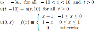
In this problem, you will solve the PDE using the method of lines as discussed in class. For all parts, use a second order central difference scheme with ∆x = 0.25 (i.e., 81 total grid points) to discretize ux. You should get a system of ODEs of the form

u′ = Au (1)

The different parts will explore different methods for solving this system.  For each part, solve from time t = 0 until time t = 3.  Each question asks you to approximate u(3, 9). This means your approximation for u at t = 3 and x = 9.

(a)  Use the forward Euler method to solve (1) with ∆t = 0.1.  Store your approxi- mation of u(3, 9) in a variable named A1.

(b)  Use the forward Euler method to solve (1) with ∆t = 0.01.  Store your approxi- mation of u(3, 9) in a variable named A2.

(c)  Use the trapezoidal method to solve (1) with ∆t = 0.1. Store your approximation of u(3, 9) in a variable named A3.

(d)  Use the trapezoidal method to solve (1) with ∆t = 0.01.  Store your approxima- tion of u(3, 9) in a variable named A4.

(e)  Use the midpoint method to solve (1) with ∆t = 0.1.  Since the midpoint method is a multi-step method, you will need to use a different method for the first time step. Use the trapezoidal method for this purpose. Store your approximation of u(3, 9) in a variable named A5.

(f)  Use the midpoint method to solve  (1)  with  ∆t  =  0.01.   Since  the  midpoint method  is  a  multi-step  method,  you  will  need  to  use  a  different  method  for the first time step.  Use the trapezoidal method for this purpose.   Store your approximation of u(3, 9) in a variable named A6.

(g)  Use the Lax-Friedrichs method to solve (1) with ∆t = 0.1.  Store your approxi- mation of u(3, 9) in a variable named A7.

(h)  Use the Lax-Friedrichs method to solve (1) with ∆t = 0.01.  Store your approxi- mation of u(3, 9) in a variable named A8.

Problem 2

Consider the initial-boundary value problem

ut  = −(0.2 + sin2(x − 1),ux   for all  0 < x < 2π and  t > 0

u(t,0) = u(t,2π)  for all  t ≥ 0

u(0, x) = cos(x)

In this problem, you will solve the PDE using the method of lines as discussed in class. For all parts, use a second order central difference scheme with ∆x = 2π/100 (i.e., 101 total grid points) to discretize ux. You should get a system of ODEs of the form

u′ = A(x)u (2)

The different parts will explore different methods for solving this system.  For each part, solve from time t = 0 until time t = 8.  Each question asks you to approximate u(4,π). This means your approximation for u at t = 4 and x = π .

(a)  Use the backward Euler method to solve (2) with ∆t = 1.  Store your approxi- mation of u(4,π) in a variable named A9.

(b)  Use the backward Euler method to solve (2) with ∆t = 0.01.  Store your approx- imation of u(4,π) in a variable named A10.

(c)  Use the trapezoidal method to solve (2) with ∆t = 1.  Store your approximation of u(4,π) in a variable named A11.

(d)  Use the trapezoidal method to solve (2) with ∆t = 0.01.  Store your approxima- tion of u(4,π) in a variable named A12.

(e)  Use the midpoint method to solve  (2)  with  ∆t  =  0.05.    Since the midpoint method  is  a  multi-step  method,  you  will  need  to  use  a  different  method  for the first time step. Use the trapezoidal method for this purpose. Store your approximation of u(4,π) in a variable named A13.

(f)  Use the midpoint method to solve  (2)  with  ∆t  =  0.01.   Since  the  midpoint method  is  a  multi-step  method,  you  will  need  to  use  a  different  method  for the first time step. Use the trapezoidal method for this purpose. Store your approximation of u(4,π) in a variable named A14.

(g)  Use the Lax-Friedrichs method to solve (2) with ∆t = 0.05.  Store your approxi- mation of u(4,π) in a variable named A15.

(h)  Use the Lax-Friedrichs method to solve (2) with ∆t = 0.01.  Store your approxi- mation of u(4,π) in a variable named A16.

Problem 3 - Relevant to the written report

Consider the initial-boundary value problem

ut  = -ux    for all  0 < x < 25 and t > 0

u(t,0) = u(t,25)  for all  t ≥ 0

u(0, x) = f(x) = e−20(x−2)2   + e− (x−5)2     for all  0 ≤ x < 25

(Note that the initial condition isn’t actually a periodic function, but u(0, 0) and u(0, 25) are so close to zero that it doesn’t really matter.)

In this problem, you will solve the PDE using the method of lines as discussed in class.  For all parts, use a second order central difference scheme with ∆x = 0.05 (i.e., 501 total grid points) to discretize ux. You should get a system of ODEs of the form

u′ = Au (3)

For each part, solve from t = 0 until t = 17 using ∆t = 1/22 (i.e., 375 total time points). At time t ≤ 17, the true solution is

u(t,x) = f((x - t)(mod25)) ≈ f(x - t)

(The exact formula is true for all time, but the approximation is only valid until one of the wave peaks reaches the boundary, which happens at some point after t = 17.)