Assignment 3

You are an analyst that evaluates equity in the Nordic region. At your disposal you have a database containing monthly stock market data on various large companies in Sweden, Norway, Denmark, and Finland. This database is dynamic and is updated each month. You have access to this database via an excel file called Assignment 3.xlsx. It contains three sheets: one with your data, one for your  input and one for your output. The sheet called Data contains the data you are to work with. The sheet called Input – where the user can specify what they are interested in – is already formatted for you. The sheet called Output is empty.

The file can access the updated data in the database via a simple click of a button in the Data sheet.1 The data uses columns A to CE (that is 83 columns). You will need to use at least columns CF to FE (i.e. 78 more columns) to extract your relevant data. As a guidance they have been colored yellow. The database uses headers in row 8 so it is recommended you do so as well. Here is what you are   tasked to do:

Part 1: INPUT

You wish to look at the state of the market in this region. To get a general idea (or to look for interesting opportunities) you wish to compare Equity (either Price, Debtor both) with Earnings (either the after-tax net income, or EBIT or EBITDA)2. This comparison between the companies’  balance sheet and their results is most often done by dividing the equity by the earnings. This is  what we aim to extract from our data.

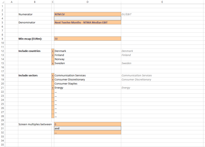
1.    In the Input sheet you are to create an easy way for even a novice excel user to specify what they wish to look for in the data. The various specifications have been labeled and the input  cells colored for easier guidance. Here is what you are to do for each:

a)    Numerator                Here we want a drop-down menu where we can choose our options

for what to have in our numerator, either Price (Market Cap), Net Debtor both (EV).3 You can find the choices in column H. Reference to them in your list.

b)   Denominator            Here we want a drop-down menu where we can choose our options

for what to have in our denominator, either E (Net Income), EBIT or EBITDA. You can find the choices in column H. Reference to them in your list.

Now we want to be able to filter our data. The various filters you need to include are:

c)    Min mcap (EURm)    Here we want to set a lower limit (in millions of euros) to the size of the companies we are looking for. Hence if we enter 50 into the cell we should not consider any companies in the database with a Market Cap lower than €50 million. You can enter a number into the cell as a placeholder for now.

d)   Include countries     Here you should list in alphabetical order, in column D, the

countries that we can look at. By putting an x in the corresponding cells in column C we decide which countries to include in our output. You can check all countries as a placeholder for now.

e)    Include sectors         Here you should list in alphabetical order, in column D, the sectors   that we can look at. You’ll find what sectors we have in our data in column J in our Data sheet. By putting an x in the corresponding cells in column C we decide which sectors to include in our output. You can check all sectors as a placeholder for now.

Lastly we might want to filter our data basedon the results we get. Since we’re looking at a  quotient,i.e. a ratio, it might not be that useful to us under some circumstances. If earnings are negative we might not be interested in comparing P/E ratios to profitable companies.

Alternatively if the earnings are very low we might be very large P/E ratios which we might wish to exclude.

f)    Screen multiples between    Here you should state a lower bound in cell D30 and an upper bound in cell D32. You can enter 0 for the lower bound and … for the upper    bound as a placeholder for now.4

2.    In order to make our choices a bit more visually intuitive and clear we will want to display

our chosen quotient in cell E3 as text. Use the relevant text in column I. For example: if we   have chosen Company Market Cap. Super Entity as our numerator and Next Twelve Months - NTMA Median Net Income - Adjusted as our denominator then in cell E3 the text P/E should appear. Use the same grey font and format as in columns H & I. (Hint: use the INDEX() and MATCH() functions to get the correct values from column I)

3.    Similarly, we wish to make clear which countries and sectors we have selected. Putting an x  in an input cell in column C should result in the corresponding name appearing in column E. Use the same grey font and format as in columns H & I. Hence column D displays our possible choices while column E displays which selections we have made. (Hint: use an IF() function to make the text appear under the correct circumstances)

Once we are finished the selection should look like this (not all sectors are shown):

Part 2: DATA

Now that you have your inputs choices in order, you need to extract the relevant values from your data. We will first extract our numerator and denominator from the data then apply our filters.

1.    First, we need to look atour data to see if all of the metrics we wish to select in our numerator and denominator are available. We goto our Data sheet and see that we have

We have 13 columns for each metric, one for each of the previous 12 months and one for   today.5  However we see that we can only find five of our six metrics. Hence we are missing one of our numerators, the EV, which was the sum of both the Market Cap and the Net Debt. So let’sadd it.

2.    We start by creating the headers for our data (in row 8). In columns CF to CQ we will have  our monthly data so we write =“NTM EV as of ” in the header. To get the correct date for    each month (since we wish to update it dynamically) we combine it with the correct dates. These can be found in our data, for example in cells S8 to AD8. Select the dates from the    rest of the text using the RIGHT() function and add them to your header using &.

Your first header, in cell CF8 should now display:

NTM EV as of 30/11/20

Create aheader that says NTM EV for the 13th  column in cell CR8.

3.    Now let’s create the metric. EV was the sum of Market Cap and Net Debt, so we just have to add the relevant cells together to get the values for our 13 columns. However, for some of

the companies in the database we have no values for either Market Cap or Net Debt.6  So the sum will return an error. To deal with this use the IFERROR() function. Have it return the sum if there is no error, otherwise it should return a blank space “ “. Double check that your

calculations are correct.

At this point it might be suitable to change your workbook from automatic calculations to manual. Goto File -> Options -> Formulas and check the box for Manual workbook

calculation. Now your numbers won’t change unless you press F9, which might save you    time since you might not want torecalculate the whole workbook each time you change a cell.7 

4.    Now that we have all of our 6 metrics we can select our numerators and denominators.

Create the headers for the numerators in cells CT8 to DF8 and for the denominatorsin DH8  to DT8.8  Create the first 12 numerator headers by referring to the relevant cell in your input sheet – they have been named for your convenience – and adding the “ as of “ and correct   date using the RIGHT() function and the & symbol. For the last one you just need to reference the cell to get the name. Do the same for the denominator.

If you’ve chosen NTM EV for your numerator and Next Twelve Months - NTMA Median EBIT for your denominator your cells CT8 and DH8 should now display:9

NTM EV as of 30/11/20

and

Next Twelve Months - NTMA Median EBIT as of 30/11/20

Fill out these columns using the INDEX() and MATCH() functions. You only need to search  row 8 for the relevant column and return the value in the relevant row – hence only two   rows are needed in your code, not the whole database. (Hint: since you’ve expanded your data by creating the EV values you should include the columns CF to CR)

5.    Next we apply our filters. Create headers for our three filters (mcap, country and sector) and in cells DV8 to DX8. Check your data for where you find a company’s country, sector and

mcap. (Hint: you can find the relevant columns early in the data) Create the filter by using

the MATCH() function to match the relevant cell to your table of selected values in column E in the Input sheet – they have been named for your convenience. If there is a match you will get a corresponding number, representing where in your table the match was found, and if   no match is found you will get an error message. Use the ISNUMBER() function to get a

true/false statement that’ll then tell you if the company should be included or not (where

TRUE means that the company should be included). You might want to use an IF() function    as well to include/exclude companies with missing values.10  Here you might want to exclude companies without a known mcapif there is a minimum, since you cannot be sure the

company has an mcap above the minimum. However you probably want to include all

companies if there is no minimum mcap – if for example the cell is left empty or if someone has entered zero as the minimum.

Lastly once you’ve successfully determined whether each company is included in each of our filter we’ll create a final fixed filter to see whether we want to include the company or not.    We includeonly the companies that are included in all three filters above. Write fixed filter    as a header in DY8 and use the AND() function to check if the three other filters all show

TRUE or not. Thus we should only get a TRUE statement in our fixed filter column if the three other columns also display TRUE.

6.    In order to create our fraction we need to have values for both our numerator and our

denominator. Since our data contains missing values we need to check for this and remove those observations from our calculations. We’ll do this in columns EA to EM. Write the header has both numerator and denominator in those columns on row 8. Check if your 13 observations have both numerator and denominator by referring to the relevant cells and using the ISNUMBER() and AND() functions. If both numerator and denominator exist, that is they have a number, your cells should display TRUE, if there are missing values it should say   FALSE. So if cells CT9 and DH9 display values the cell EA9 should say TRUE, if at least one of   those two cells are empty (i.e. missing a value) the cell EA9 should say FALSE for that row.

7.    We can now calculate our multiples. In cells EO8 to EZ8 you can write multiple as a header. For the cell FA8 you can write latest as the header since this is most current value.11

Calculate the 13 multiples by

a.    Checking the fixed filter column to see if they should be included and the relevant  has both numerator and denominator column to see if the quotient exists. Use the AND() function. It should say TRUE if there is a quotient that passes our filter.

b.    Use an IF() function to either give the quotient,i.e. divide the relevant numerator by the relevant denominator, or return a blank space “ “ depending on the outcome of  the AND() function. If your AND() returns TRUE then we should get the quotient, if     FALSE then we should get an empty cell.

c.    Lastly use IFERROR to change any error message to a blank space “ “ .

The cells in your multiples and latest columns should now either display values or be empty.

8.    Lastly we apply our output filter where we screen our multiples and only keep those within the bounds we’ve chosen in our Input sheet. We’ll only test ifour latest multiple is within    our bounds.12  In cells FC8 to FE8 write the headers lower, upper and latest filtered respectively. Calculate if your latest multiple is within your lower bound by

a.    First checking if the bound exists, do so using the ISNUMBER() function and referring to the relevant cell in your Input sheet.

b.    If the lower bound exists we check if we are above it, but otherwise we don’t need  to worry so use the NOT() function on your ISNUMBER() statement. This will return the opposite of what you previously had (it’s as if you used a ISNOTNUMBER() function)

c.    Now we know our latest multiple complies if either our lower bound doesn’t exist   (which would result in our NOT() function returning a TRUE statement) or if it the    multiple is greater than or equal to our lower bound (i.e. if the statement: multiple >= our lower limit returns the value TRUE) . Use the OR() function to check these two criteria since if either is TRUE then you are fine.13

Calculate the cells for your upper bound using the same functions but comparing your latest multiple to the upper bound and seeing if it is below it (i.e. use the statement: multiple <=     our upper limit).

If you’ve done both correctly then if the multiple in the latest column is within the bounds then both the upper and lower column cells on the same row should display TRUE.

In your latest filtered column use the IF() and AND() functions to determine if both the upper and lower bound columns display TRUE and, if that is the case, the latest filtered column

should display the value from the latest column, if not, it should return a blank space “ “ .

Part 3: OUTPUT - AGGREGATE

We’ve now created a selection process where we choose what we want in our Input sheet and away to extract what we want into our Data sheet. What remains is to structure this data into relevant dynamic tables and graphs that can be used by a less experienced user to look for interesting aggregate information. We’ll do this in our Output sheet.

1.    We will calculate our sector wide aggregates. Write Numerator in boldin cell B2. Create a

table with headers from cells C3 to O3 with the dates from the Data sheet. Remember,

these need to be dynamic references that change from update to update so plaintext wont   do.14 Also, it is preferable to have excel understand that they are dates so you should make    sure that they are treated as such in the sheet.15  Make sure to order the dates from oldest to newest with the mostrecent date (in this case: 22th  Nov 2021) in cell O3. In cells B4 and

down put your different sectors, sorted in the same order as in your Input sheet, and below   them create a category called Market that’ll represent all selected sectors.16  Use appropriate formatting to make the market row distinct from the individual categories.

Put in the correct values for each industry for each date. These are the numerators (which     represent value of equity / debt) so adding alltogether is reasonable. Use SUMIFS to get the correct values. Format the cells to have no decimals. Sectors that are not included in the filter should result in empty rows.17  (Hint: you need to check not just the industry and date but also that it is included in the filter and that both the numerator and denominator exist; and remember to use fixed or mixed references when appropriate!)

2.    Create a similar table for the denominator below the first one. Write Denominator in boldin  cell B17 and put the dates in cells C18 to O18 and the industries (and Market) in cell B19 and down.

3.    Now we’ll create our table of quotients. Write Aggregate in boldin cell B32 and put the

dates in cells C33 to O33 and the industries (and Market) in cell B34 and down. Format the cells to have only use one decimal and to have an x after it (i.e. the cells should display

something like 13.2x) to indicate that these are factors.18  Take note with how you calculate the Market values! Make sure to leave excluded industries blank. (Hint: use the IFERROR()   function)

4.    Sometimes it is hard to get an idea of how much aggregated values represent most

companies or instead a few outliers. In order to get another metric for how the market is doing is to look at the median. So we’ll create atable that shows the median of all these  industries. Write Median in boldin cell B47 and put the dates in cells C48 to O48 and the industries (and Market) in cell B49 and down.

Calculate the medians for the relevant sector and date using the MEDIAN() and IF()

functions. Note that if you get a correct answer in the preview of your function box but the actual cell returns a #VALUE! error then you need to create an array in your calculations. Do this by pressing ctrl + shift + enter when you are done instead of just enter as you would otherwise do.19  Use the IFERROR() function to deal with filtered out sectors. Take note with

how you calculate the Market values! (Hint: remember that you have calculated the individual multiples in your Data sheet already)

5.    Now we will make a few graphs where we compare two industries to each other and to the   market. Write Graphs in boldin cell B62 and put the dates in cells C63 to O63. In each of the cells B64 and B65 create a drop down menu where you can choose an industry.  Use the

INDEX() and MATCH() functions to get the relevant data from your Aggregate table into cells C64 to O65. In Cell B66 write Market and put the aggregate market factors in cells C66 to

O66.

Create a similar table on rows 69 to 71 that uses the relevant data from your Median table.  Use drop down menus in cells B69 and B70 and have Market in row 71.20  Give the cells with the drop down menus the same color as our input cells in the Input sheet.

Lastly write Market Aggregate and Market Median in cells B74 and B75 respectively and include the relevant data in the rows.

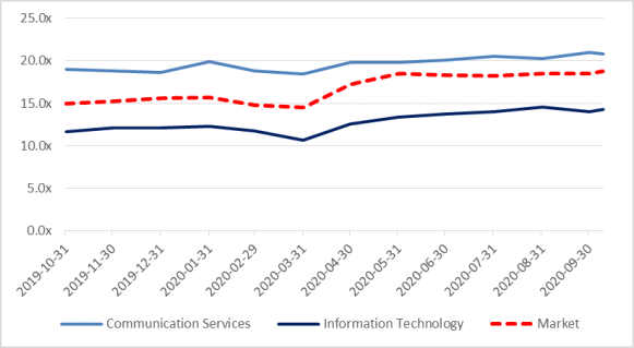
We wish to create three graphs with the same layout. The easiest way to do this is to create the first graph, format it and then make copies that keep our format. We then just change

the data references in the graph. Create a line graph that links to your table in rows 63 to

66. Change the colors of the lines so that one sector is light blue and the other dark blue.

Change the color of the line representing the market to red and make it a dashed line.21  Now it should look something like this:

Now create two copies and put the three graphs next to each other in using rows 79 to 93. Change the other two graphs to refer to the Median data and the Markets Aggregate and   Median respectively.22

6.    We’ll also make some sorted bar charts23  to see where the various sectors fall compared

each other and to the market according to our latest figures. In cells A96 and down write 1, 2, 3 etc for all your sectors (not just the selected ones!) plus the market. In cells C96 and

down sort your latest aggregate numbers from largest to smallest using the LARGE() function. (Hint: you can refer to the values in column A to get your position)

Use the INDEX() and MATCH() functions in column B to get the sectors corresponding with the values in column C. Write blue in cell D95 and red in cell E95. Use the IF() function in

column D to display the values in column C if the name in column D is not Market. Use the opposite criterion in column E.24  Now your blue column should display all the aggregate

factors for the selected sectors while you red column should only display the aggregate factor for the Market.

Use the IF() and IFERROR() functions to get rid of any error messages.

Create a bar chart using stacked columns. Use Select Data to adjust it so that your names in  column B appear on your horizontal axis and the data in columns D and E are in your graph. In the default settings your sectors should appear blue and your market red, if not then change the graph so that it does. Put the graph in row 109 and down. It should look like this:

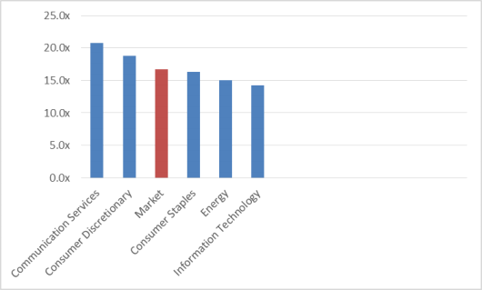
There will be a blank space to the right by design if you’ve not selected all sectors on your Input sheet.

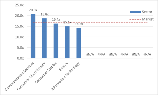
7.    Repeat what you did in columns B to C in the columns G to H respectively for rows 96 and down. However, in column H, exclude Market from the sorted list and display the error

message #N/A for missing values.25  Column G should now be identical to Column B except for the absence of Market.26  In column I display the aggregate factor of the market. Write  Sectors in cell H95 and Market in cell I95.

Create a bar chart with a line through it using combo chart. In the default settings the

sectors should be bars and the market should be a line, if not then change the graph so it is. Change the market line to a dashed line and reduce its weight to 1.5 points.27  Display the

values on top of the bars by clicking on them and using Add Chart Element -> Data Labels -> Outside End. Your chart should now look like this: