ECE / CS 6501: Geometry of Data

Hello, dear friend, you can consult us at any time if you have any questions, add WeChat: daixieit

ECE / CS 6501: Geometry of Data

Homework 2: Geodesics and Manifold Statistics

Instructions: Submit a single Jupyter notebook (.ipynb) of your work to Collab by 11:59pm on the due date. All code should be written in Python and math formatted in LaTeX inside the notebook. Be sure to show all the work involved in deriving your answers! If you just give a final answer without explanation, you may not receive credit for that question.

You may discuss the concepts with your classmates, but write up the answers entirely on your own. Do not look at another student’s answers, do not use answers from the internet or other sources, and do not show your answers to anyone.

1 Geodesic Equation on S²

In this problem, you will compute the geodesic equation on the 2D sphere. Consider the standard (θ, φ) parameterization of the sphere:

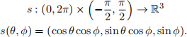
Throughout this problem, you will use this (θ, φ) coordinate system. These coordinates correspond to the notation (x1, x2) in the notes for a generic 2D manifold. Anywhere you may see integer indices in the notes, you might replace them with θ, φ. For example, the Christoffel symbol  could be written as .

(a) Write down equations for the coordinate tangent vectors  and . Hint: These should be vectors in R³ that are functions of θ, φ, and they are computed by just taking the partial derivatives of the equation for s(θ, φ).

(b) Using the induced metric of R³, write down the coefficients of the Riemannian metric, g, on S2 in terms of the coordinates θ, φ. Hint: You should end up with a 2 x 2 matrix, whose entries are functions of θ, φ and are just Euclidean R³ inner products of the tangent vectors from the previous part.

(c) Compute the inverse metric g⁻¹. Again, this will be a 2 x 2 matrix whose entries are functions of θ, φ.

(d) Compute formulas for the Christoffel symbols, .

(e) Show that the equator circle γ(t) = s(t, 0) is a geodesic.

(f) Provide an argument that all great circles (circles on S² with radius = 1) are geodesics. You don’t need a lengthy or precise proof, just a brief and informal argument will suffice.

2 Statistics on Shape Manifolds

In this project you will implement Kendall’s shape space and simple shape statistics, namely, the Fr´echet mean. You first must decide on a data structure for representing a 2D point set (called an“object” throughout this assignment). For an object containing n points, you may decide to use either an 2 x n real matrix or a list of n complex numbers. Also, you will want to have a way to plot your resulting shapes.

Methods: You will need to implement functions that perform the following operations:

1. Project an object onto the preshape sphere by removing its centroid and scaling it to unit norm. This is a preprocessing step that all objects will go through before applying any of the following routines.

2. Perform Ordinary (a.k.a. Orthogonal) Procrustes Analysis (OPA). This should input a target preshape and moving preshape and output the aligned version of the moving preshape.

3. Compute the exponential map on Kendall shape space, i.e., given a preshape and tangent vector, compute the preshape at the end of the corresponding geodesic.

4. Compute the log map on Kendall shape space, i.e., given two preshapes, compute the tangent vector at the first preshape that is the initial condition of the geodesic segment between the two.

5. Estimate the Fr´echet mean shape using gradient descent as described in class.

6. Compute the approximate principal geodesic analysis (PGA), that is, perform principal com-ponent analysis (PCA) in the tangent space to the Fr´echet mean.

Experiments: You will test your shape analyis routines using two datasets: one synthetic and one from real images.

1. Random triangles. Generate a set of 100 triangles with the following three points:

where s is a Gaussian random variable with mean 1 and standard deviation 0.5. Next, add zero-mean Gaussian noise with s.d. 0.1 to all six coordinates of each of the 100 triangles.

2. Corpus callosum shapes: https://tomfletcher.github.io/GeometryOfData/homeworks/cc-shapes.zip Each corpus callosum object consists of 64 points listed in an ASCII text file. Each line of the file contains a single point (x and y coordinates).

Report: You should discuss your work in your Jupyter notebook. Be sure to include the following:

● Describe your implementation. You do not need to recount the theory and equations behind all of the methods, just a brief description of how you implemented them and the issues you faced.

● Describe both the triangle and corpus callosum experiments. For each experiment include:

– Pick two objects from the data set and plot a geodesic between them (this should be a sequence of objects deforming from one to the other).

– Plots of 1) the raw object data (i.e., all points from all objects overlaid in one plot), 2) the preshapes aligned to the Fr´echet mean, and 3) the Fr´echet mean shape (in a different color). Can you see an obvious difference in the aligned shapes?

– A plot of the eigenvalues for each mode (scree plot). Looking at this plot, how many modes would you use to describe the data?

– Plot the modes of variation at 0, ±1, ±2 standard deviations. You only need to plot up to 3 different modes (maybe fewer, if you decided in the previous question that fewer were needed to represent the data).

– Describe what you are seeing in the modes of variation. For the triangle case, is this the variation you expected?

● Discuss: What is the maximal number of modes that are possible for triangle shapes? In general, what are the maximal number of modes that are possible for a set of objects with n points?