关键词 > ECOM30002/ECOM90002
ECOM30002 / ECOM90002 Econometrics 2 Semester 2 Assessment, 2021
发布时间:2023-11-10
Hello, dear friend, you can consult us at any time if you have any questions, add WeChat: daixieit
Semester 2 Assessment, 2021
Faculty / Dept: Faculty of Business and Economics / Department of Economics
Subject Number: ECOM30002 / ECOM90002
Subject Name: Econometrics 2
Writing time: 3 hours
Reading time: 30 minutes
Number of pages (including this page): 7
Paper to be held by the Baillieu Library: No
Open Book Status: Yes
Instructions to Students
You have 3.5 hours to complete this exam from when you commence. This includes the reading time. Canvas logs will be used to confirm that the 3.5 hours have been adhered to. Please use a timer to monitor the allotted time.
You are allowed to use notes, textbooks or resource materials, as authorised by the Board of Examiners.
You can access an Exam Support Chat tool for the first 45 minutes of the exam. Please log your concern via the Canvas chat board in the first instance using the Big Blue Button. Alternatively, you can call the following numbers for assistance during the exam if you are experiencing technical difficulties. Inside Australia: 13MELB (13 6352) (select Option 1 for current students then select Option 1 again for exam enquiries). Outside Australia: +61 3 9035 5511 (select Option 1 for current students and then select Option 1 again for exam enquiries)
You will be able to contact your examiner during the examination reading time. Do not contact your lecturer during the examination period.
Your answers must be submitted as a single PDF file using the LMS assignment tool. Your name and student number, the subject code and the subject name must appear on the first page of your submission. Your student number must appear onevery page. Question numbers must be clearly indicated in your answers.
Your answers may be either fully word-processed, fully handwritten or a mixture of the two. If you wish to submit any handwritten content, then it must be scanned and included in your PDF. You must include your student number on every page of scanned content.
This exam contributes 70% to the final subject mark.
This exam has SIX questions, worth 20 marks each, for a total of 120 marks. Answer ALL questions.
Question 1 (20 marks )
A country has been ravaged by a pest. The economy is struggling, with 3 of the country’s 6 equally large economic sectors set to end the financial year with losses. The government is considering a reform package, but it would have heterogeneous effectson the economy.
The following table characterises the potential outcomes of the reform, where Y1i denotes sector i’s potential profits (for Y1i > 0) or losses (for Y1i < 0) if it were subjected to the reform, and Y0i denotes i’s potential profits or losses if it were not subjected to the reform:
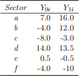
Consider the following three different ways of assigning the treatment:
(i) the reform applies to every sector in the economy;
(ii) adoption of the reform is voluntary (assume that each sector acts as a single profit-maximising
agent that has perfect information of the sector’s potential outcomes);
(iii) the reform only applies to sectors set to post a loss without the reform.
1. ( 6 marks) What is the average effect of the treatment on the treated (ATT) for each case (i), (ii), and (iii)?
2. (3 marks) Does any of the three ATTs above correspond to the average treatment effect (ATE)? Explain.
3. ( 5 marks) Calculate the OLS coefficients for the regression of Yi on Xi for case (iii).
4. ( 6 marks) Calculate the selection bias for case (iii), and give an intuitive explanation of why the OLS regression does or does not estimate a causal effect in this case.
Question 2 (20 marks )
A researcher is interested in the effect of family size on mothers’ employment.
Specifically, the researcher uses a sample of women with either two or more children to estimate the causal effect of a third birth (ThirdBirth i=1 if mother i has three or more children, 0 if she has two) on whether the mother is employed (Employed i=1 if i is employed, 0 otherwise). The instrument used for third birth is an indicator of the second birth being twins (Twins i=1 if mother i’s second and third children are twins, 0 otherwise).
The researcher reports the following results.
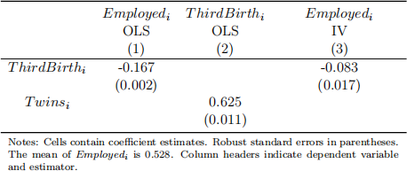
1. (2 marks) Give an appropriate interpretation of the OLS estimate from Column (1).
2. (4 marks) Explain why the OLS estimate is unlikely to represent the causal effect of hav- ing more than two children on employment for the population in question, giving concrete examples that apply to this setting.
3. (4 marks) Interpret the estimated first stage slope, and calculate the first stage intercept.
4. (4 marks) Do the results indicate that the instrument is relevant? Explain your answer. Based on theory, is this result surprising? Explain your answer.
5. (4 marks) Do you think the instrument is exogenous? Explain why or why not.
6. (2 marks) Give an appropriate interpretation of the IV estimate from Column (3).
Question 3 (20 marks )
Consider the following system of equations:
where E(U1ij Z1i, Z2i) = 0, E(U2ij Z1i, Z2i) = 0, E(U3ij Z1i, Z2i) = 0.
1. ( 7 marks) Let α13 = 0, and α12 ![]() 0, α21
0, α21 ![]() 0. Carefully explain under which conditions equations (1) and (2) are identified and how one could estimate the parameters.
0. Carefully explain under which conditions equations (1) and (2) are identified and how one could estimate the parameters.
2. ( 7 marks) Let α21 = 0, and α13 ![]() 0, and α12
0, and α12 ![]() 0. Explain under which conditions OLS estimation of (1) is inconsistent. Stating any necessary assumptions, explain if and how one could estimate the parameters of (1) in that case. Distinguish between the cases of β11 = 0 and β11
0. Explain under which conditions OLS estimation of (1) is inconsistent. Stating any necessary assumptions, explain if and how one could estimate the parameters of (1) in that case. Distinguish between the cases of β11 = 0 and β11 ![]() 0.
0.
3. ( 6 marks) As in part 1 of this question, let α13 = 0, and α12 ![]() 0, α21
0, α21 ![]() 0. Suppose i indexes cities, Y1i represents the number of murders per capita, and Y2i represents the number of police officers per capita. Explain if the simultaneous equations system (1)-(2) is well-defined in the sense of each equation having its own clear causal interpretation. What signs for α12 and α21 do you expect and why?
0. Suppose i indexes cities, Y1i represents the number of murders per capita, and Y2i represents the number of police officers per capita. Explain if the simultaneous equations system (1)-(2) is well-defined in the sense of each equation having its own clear causal interpretation. What signs for α12 and α21 do you expect and why?
Following a terror attack in a neighbouring country, the federal government announces it will strengthen national security by spending more on safeguarding big cities. Which variable in the model do you think would best represent these extra funds? Based on your answer, discuss whether this variable would help identify any (or all) of the equations in the system.
![]() Question 4 (20 marks )
Question 4 (20 marks )
Consider the following panel data generating process (DGP), from which 10,000 repeated samples were drawn of n = 100 cross-sectional units i observed over T periods of time; i.e., t = 1, 2, . . . , T :
Yit = βXit + Uit , where Uit = αi + Vit , (4)
where each Xit and Vit were drawn from two independent standard normal distributions, Xit
N(0, 1) and Vit N(0, 1); and αi = δX(-)i + εi , with εi N(0, 1) and X(-)i = ![]()
![]() Xit.
Xit.
Throughout the simulation, β = 1. The simulation is repeated for the four different combina- tions of δ = f0, pT g and T = f2, 8g (the four combinations are listed in the table below). In each repeated sample, model (4) is estimated by pooled OLS (“Pool”) and by the fixed effects estimator (“FE”). For each estimate of βE obtained with estimator E = fPool, F Eg, a t-test is conducted using the test statistic
where rse(β(ˆ)E ) denotes a heteroskedasticity-and-autocorrelation-consistent (HAC) standard error ofβ(ˆ)E . The following table summarises the results obtained from the simulation:
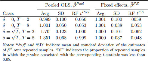
1. (2 marks) Show that for both values of δ (0 and pT) the variance of αi does not depend on the number of time periods T.
2. ( 6 marks) Explain in which of the four cases pooled OLS and FE are unbiased for β, and in which they are biased.
3. ( 6 marks) Discuss the estimated standard deviations of the estimators (SDs), by linking observed differences in the SDs to features of the DGP and of the estimators.
4. ( 6 marks) For all four cases, interpret the reported rejection frequencies and comment on whether they are consistent with your expectations regarding the size and/or power of the test.
Question 5 (20 marks )
In Australia, the government uses a number of financial incentives to bolster the uptake of private health insurance (PHI). Rich individuals face a negative incentive payment (a tax penalty) called the Medicare Levy Surcharge (MLS) if they do not purchase PHI. Eligibility for the MLS is a function of the individual’s taxable income, with the threshold having changed a number of times in the past. Consider the following panel data model for the demand for PHI:
PHIit = ρPHIit-1 + βMLSMLSit + Xi(地)tβ + αi + t + Vit , (5)
where PHIit is a dummy indicating that individual i in year t had purchased PHI, and MLSit is a dummy indicating that i in t was eligible for the MLS. Xit is a vector containing individuals’ age, income and self-assessed health status.
1. (4 marks) Explain which parts of Equation (5) can reflect persistence in the demand for PHI beyond that explained by Xit and how the persistence induced by these parts differs from each other.
2. ( 6 marks) A group of individuals becomes temporarily eligible for MLS in year t (they are ineligible in all other periods). What is the effect of this temporary eligibility on the demand for PHI in years t, t + 1 and t + 2 if (i) ρ = 0? (ii) ρ ![]() 0?
0?
Now consider the following table of estimation results for variants of (5):
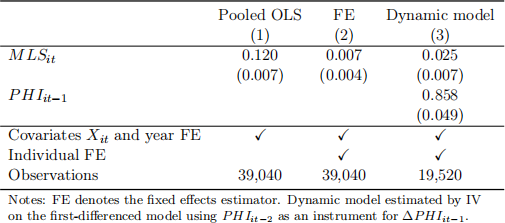
3. (4 marks) Consider only the results in columns (1) and (2). What does the difference between the Pooled OLS and FE estimates of the coefficient on MLS reveal about the effect of omitted individual-specific variables on the demand for PHI and their relation to MLS?
4. ( 6 marks) Is the FE estimator consistent if ρ ![]() 0? Explain and discuss which of the three estimators in the table is your preferred estimator based on the reported results and why.
0? Explain and discuss which of the three estimators in the table is your preferred estimator based on the reported results and why.
This question considers quarterly time series data from the first quarter (q1) of 1987 to the fourth quarter (q4) of 2013 for Australian domestic beer sales (Beer t, index value equal to 100 in the first quarter of the year 2000) and domestic wine sales (Wine t, also indexed to 100 in q1 of 2000). The real growth rates for the variables are gBeert = 400Δ log Beer t and gWine t = 400Δ log Wine t , respectively. The table below contains estimation results for some autoregressive (AR) models for gBeert with a maximum lag order of 4.
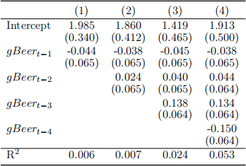
1. ( 7 marks) Making reference to the results in the table, explain why R2 should not be used for lag order selection for AR models. In contrast, explain conceptually how the Akaike Information Criterion (AIC) works for lag order selection.
Consider the following results from two ARDL models (left-hand-side table), as well as index values of Beer t and Wine t over the four quarters of 2013 (right-hand-side table):
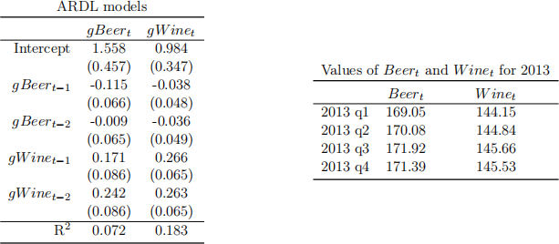
2. ( 6 marks) Explain how an ARDL model differs from an AR model. What is the information set used to estimate the ARDL model for gWine t? How does it differ from the information set used to estimate the ARDL model for gBeert, if at all?
3. ( 7 marks) A friend of yours forecast gWine t for q1 of 2014 as 1.154. Use the available information to forecast the values of gBeer t in q1 and q2 of 2014.
