关键词 > EEEN4/60161
EEEN4/60161 Digital Image Processing LABORATORY 3 (2023/24)
发布时间:2023-11-07
Hello, dear friend, you can consult us at any time if you have any questions, add WeChat: daixieit
EEEN4/60161 Digital Image Processing LABORATORY 3 (2023/24)
Objectives:
. Understand and practise frequency-domain image processing
. Understand block-based image processing and DCT-based image coding
Equipment: Matlab, Simulink, Computer Vision Systems Toolbox, Image Acquisition Toolbox, camera, tripod.
Introduction
Spatial frequency is an important concept in image processing and vision. Frequency-domain image processing involves 2D Discrete Fourier Transforms (DFT) and filtering images in the frequency
domain. In first part of this laboratory you will first practise 2D DFT (forward and inverse) and
appreciate the meaning of spatial frequencies, before practise lowpass and highpass filtering in the frequency-domain.
Block-based coding may not be the best way to code image data but it is simple, relatively easy to
implement. For these reasons it is widely used in existing and commercial image codecs. In the
second part of this laboratory you will explore the properties of block-based processing, especially the Discrete Cosine Transformation (DCT) that is widely used in image coding. The DCT is a
reversible transformation, that is, the transformed can be reversed to provide an exact replica of the input image. For efficient coding we abandon the requirement that the input be transmitted exactly and seek only a good approximation to the input. This process is known as lossy coding. In this lab the image quality will be evaluated for representations using different numbers of DCT coefficients.
Procedure
1. Frequency Domain Processing
1.1. Spatial frequencies
(1). Generate a 128-point sine wave/sequence as follows:
clear;
n=1:128;
x=sin(2*pi*n./16); % i.e. f=fs/16; format: 2*pi*f*n/fs
figure();plot(x);
% Apply (1D) DFT (Matlab function: fft) to the signal and display the magnitude spectrum:
y=fft(x); %do a 128-point DFT
figure(); plot(abs(y)); % magnitude spectrum, uncentred, 0(DC) to fs
% You can centre the spectrum, so spectrum is from -fs/2 to fs/2, with dc at the middle point:
figure();plot(abs(fftshift(fft(x))));
Can you see that f = fs/16 or fs is 16 times off from the spectrum? If not, discuss with the staff.
[Note. fs is the sampling frequency, inverse of the sampling period, the interval between two
consecutive samples), say Ts (whose value isn’t known in this case, let’s just note it as Ts). As the sine wave here is generated with setting its f = fs/16. The DFT analysis on its generated sequence should
reveal this relationship. Entire points (128) of the spectrum span by fs. In this case, there is a peak at the 8th point (uncentred) denoting the frequency o the signal. So, fs = 16xf, orf =fs/16. In real signal
analysis, we would know the sampling frequency, e.g. Ts=44.1kHz for audio signals, then you can work out the exact frequencies in Hz of the signal.]
(2). Extend the signal x in (1) to 2D, i.e. an image (call it X), by the following:
for i=1:128
X(i,:)=x;
end
Now, X is an image of 128x128 pixels with each (horizontal) line being a sine wave. So it is a set of vertical bars of sine waves.
Display the image. Apply 2D DFT (Matlab function: fft2) to analyse its magnitude spectrum (uncentred and centred) and spatial frequency (horizontal) in respect to size of the image.
[Note, here horizontally points in X are treated as pixels and assume the gap between consecutive pixels is Ts (whose unit is mm or angle, its inverse is the horizontal sampling frequency fs), then the analysis
should reveal a peak at the 8th point of the first row of the 2D DFT (spectrum), which is 16th of the entire spectrum, i.e. fs, the horizontal sampling frequency.]
Vary the fs/f ratio in x (and soX) from 16 to 8 and 4, generate the signal and image again and plot the spectra again to appreciate the relationships.
1.2. Forward and inverse 2D DFT
(1). Recreate the example of 2D DFT in page 5 of the lecture handouts. First generate an image of a small white rectangle in black background with the code given. Display the image. Then
perform 2D DFT and display the magnitude spectrum. Centre the spectrum, and display in logarithm scale.
(2). Load a real image (e.g. [I,map]=imread('lena_gray.png');) (image Lena of 512x512 8-bit grey scale: lena_gray.png, available on Blackboard, under Laboratory (Lab 3). Then display the image (e.g. imshow(I, map);). Perform 2D DFT on the grey level image (e.g. after, X=ind2gray(I,map)) and display the magnitude spectrum. What can you see
from the spectrum (uncentred, centred, and/or log scaled)? Discuss with staff if you wish.
(3). Now apply the inverse 2D DFT (Matlab: ifft2) on the raw spectrum and display the result. Is it the same as the original image?
Try to recover the image in (1) by applying the inverse 2D DFT to the spectrum of (1). Is the recovered image different from the originally generated image? Why?
1.3. Frequency-domain image filtering
(1). Based on the definitions (formulae in following table) on the lecture notes (section 8.4), generate the ideal and Butterworth or Gaussian filters, respectively, with the cut-off
frequency D0 set to 40.
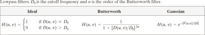
Note: D(u,v) = [(u-M/2)2+(v-N/2)2]1/2 , imagesize: M ×N, n is the order of the filter, e.g. n=2.
Plot the generated filters (i.e. their frequency response). Are they as you expected?
(2). Apply these filters to the Lena image in the frequency domain, respectively.
f (x, y)* h(x, y) ![]() F(u, v)H(u, v)
F(u, v)H(u, v)
That is, multiply the spectrum of the image with the filter’s frequency response (element by
element) and then apply inverse 2D DFT. Display the filtered image (inverse of the multiplied spectrum), respectively. What is the effect of the filtering? Comment on the differences of these different filters.
(3). (Optional) Convert these filters to high-pass filters (again using D0=40). Refer to the
lecture notes for the definitions of these filters. Then apply them to the Lena image (in the
frequency domain). What are the effect and differences among them? With this in place, you should be able to design and apply the homomorphic filtering to enhance the part affected by poor illumination (to some extent).
2. Image Coding
2.1. Block processing
Simulink provides a model called “Block Processing” to allow an input image to be divided
into smaller blocks for processing andre-assembled. Setup the system below as a model.

The video input block can be found in the Image Acquisition toolbox and the block processing block and video display block are from the CVST. Set the video device to 640x480 resolution and YCbCr output (with separate colour signals). Click the “show subsystem” option on the
block processing to confirm that the processing is “straight through” (i.e. no change should be introduced by the encoder or decoder). The default simulation time is 10 seconds –you should set this to something longer (say 100 seconds). Now run the model and confirm image display. If you do not have a USB camera or if it is not supported, you can use an image file as input, e.g. grey scale Lena image (Lenatif image, also set its output data type to double).
Next introduce some distortion into the encoder stream using the subsystem below in the encoder block
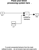
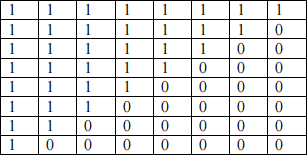
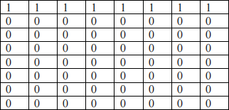
The block marked 8x8 is a constant matrix. Set the upper triangle of the matrix to ‘1’ and the upper triangle to ‘0’. This is achieved by using ‘;’ to delimit rows. For example:
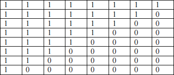
would be represented by: [1 1 1 1 1 1 1 1; 1 1 1 1 1 1 1 0; 1 1 1 1 1 1 0 0; 1 1 1 1 1 0 0 0; 1 1 1 1 0 0 0 0; 1 1 1 0 0 0 0 0; 1 1 0 0 0 0 0 0; 1 0 0 0 0 0 0 0]
Now run the model. Observe the output image and explain any distortion visible. You could vary the matrix by changing its numbers and observe the output images, for examples, using more ‘ 1’s or more ‘0’s, or using different ‘ 1 ’ and ‘0 ’ patterns.
2.2. DCT-based coding
Now setup DCT encoder and decoder subsystems as shown below (the constant ‘ 128 ’ should be 0.5 in the new version of the toolbox).
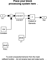
(i) Encoder
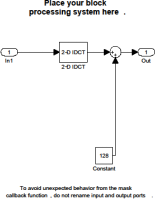
(ii) Decoder
The 2-D DCT block can be found in CVST. Set the 8x8 constant matrix to all ‘1’s so that all DCT coefficients are transmitted without distortion. Now run the model and confirm correct
output. This is straight through, so no distortion should be expected. If any of the 8x8 constant matrix is set to ‘0’, then corresponding DCT coefficients are discarded and resulting decoded image is degraded (maybe visually noticeable or not, depending on which coefficients are
discarded). Experience this and find out from the output.
Amend the model from to give a numerical display of PSNR (PSRN block is available from CVST) and measure the PSNR for different scenes. Now introduce some approximation into the system by setting some elements of the constant matrix (e.g. the upper triangle) to zero.
Observe the image quality. Produce a plot of the PSNR values and comment on the subjective image quality
2.3. DCT with different numbers of coefficients
For this part the input image should remain constant. Ideally the image should be full of content. Carefully fix the camera position –if the camera is allowed to move then your results maybe
invalid. Use the Simulink model above to calculate the variation in PSNR for different
numbers of horizontal and vertical DCT coefficients. For example, the following two types of matrix:
Type-I: (upper-left triangle with “1” and lower-right triangle with “0”),
With representation: [1 1 1 1 1 1 1 0; 1 1 1 1 1 1 0 0; 1 1 1 1 1 0 0 0; 1 1 1 1 0 0 0 0; 1 1 1 0 0 0 0 0; 1 1 0 0 0 0 0 0; 1 0 0 0 0 0 0 0; 0 0 0 0 0 0 0 0]
You can start with single ‘1’ in the top-left (set the rest to ‘0’); then add the second diagonal ‘1’s; … and so on; to fully 15 diagonal lines of ‘1’s. Measure the PSNR of each case (on the same fixed scene) to compare the effect. You can also explore the effect by adding ‘1’s
gradually from top-left corner in zigzag – similar to the quality control used in JPEG coding.
Type-II: (upper-left triangle with “0” and lower-right triangle with “1”), rarely used in any scheme, only to appreciate the high frequency elements.
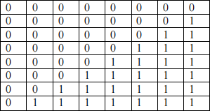
With representation: [0 0 0 0 0 0 0 0; 0 0 0 0 0 0 0 1; 0 0 0 0 0 0 1 1; 0 0 0 0 0 1 1 1; 0 0 0 0 1 1 1 1; 0 0 0 1 1 1 1 1; 0 0 1 1 1 1 1 1; 0 1 1 1 1 1 1 1]
Vary the number of diagonal lines of “1” to see the effect in this type of matrix. Plot PSNRs against the number of coefficients (or diagonal ‘1’s), observe the effect.
You could also experiment other types of matrix such as varying the number of vertical columns of “1” or the number of horizontal rows of “1” .
2.4. DFT-based coding (optional)
If time permits repeat section 2.3 of this experiment using the Discrete Fourier Transformation (DFT). The 2-D FFT block is in CVST. Is this transformation as effective when the coefficients are selected as before?
2.5. Effect of horizontal or vertical coefficients (optional)
If time permits repeat section 2.3 of this experiment but with the coefficients in horizontal or vertical rows (instead of diagonal ones), or in mirror-image sets, as the one shown below for example. Again, these are rarely used in practice, only to appreciate the effect.
3. Reporting
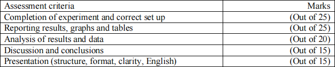
Produce a brief report up to 6 pages (excluding cover page and appendix) summarising your
experiments (sections 1.3 and 2.3), observations, key results and conclusions. Describe your
modification to measure and display PSNR. Present clear plots of PSNR for different numbers of coefficients. Discuss the reason for any difference in the number of coefficients needed in the
horizontal and vertical directions. Suggest the most effective coding transformation based on your results. Additional results can be included in Appendix.
Suggested structure:
Cover page with course/experiment, name and registration number
1. Introduction (e.g. objectives and applications)
2. Experiments (sections 1.3 and 2.3), results and analysis
3. General discussion and conclusions
Submit your report (preferably in pdf file) to the Blackboard before the deadline. Please name your report file meaningfully, e.g. DCTlab-xxxxxxx.pdf, where xxxxxxx is your ID number.