COSC2500/COSC7500—Semester 2, 2023

Hello, dear friend, you can consult us at any time if you have any questions, add WeChat: daixieit

COSC2500/COSC7500—Semester 2, 2023

Exercises—due 3:00 pm Friday 27th October

Required

The grade of 1–5 awarded for these exercises is based on the required exercises. If all of the required exercises are completed correctly, a grade of 5 will be obtained.

R4.1 Do either part (a), (b), or (c) below. (If you want to do more than one of these, see the additional exercises!) These are Q1 in Sauer computer prob-lems 8.1, 8.2, and 8.3.

a) From Sauer 8.1: Solve ut = 2uxx for 0 ≤ x ≤ 1, 0 ≤ t ≤ 1, for the sets of boundary conditions

i. u(x, 0) = 2 cosh x for 0 ≤ x ≤ 1

u(0, t) = 2 exp(2t) for 0 ≤ t ≤ 1

u(1, t) = (exp(2) + 1) exp (2t − 1) for 0 ≤ t ≤ 1

(Solution is exp(2t + x) + exp (2t − x))

ii. u(x, 0) = exp x for 0 ≤ x ≤ 1

u(0, t) = exp(2t) for 0 ≤ t ≤ 1

u(1, t) = exp(2t + 1) for 0 ≤ t ≤ 1

(Solution is exp(2t + x))

using the forward difference method for step sizes h = 0.1 and k = 0.002. Plot the approximate solution (the mesh command might be useful). What happens if you use k > 0.003? Compare with the exact solutions.

HINT: You can use Program 8.1 (heatfd.m) from Sauer.

b) From Sauer 8.2: Solve the following initial–boundary value problems using the finite difference method with h = 0.05 and k = h/c. Plot the solutions.

i. utt = 16uxx

u(x, 0) = sin(πx) for 0 ≤ x ≤ 1

ut(x, 0) = 0 for 0 ≤ x ≤ 1

u(0, t) = 0 for 0 ≤ t ≤ 1

u(1, t) = 0 for 0 ≤ t ≤ 1

(Solution is u(x, t) = sin (πx) cos(4πt))

ii. utt = 4uxx

u(x, 0) = exp(−x) for 0 ≤ x ≤ 1

ut(x, 0) = −2 exp (−x) for 0 ≤ x ≤ 1

u(0, t) = exp (−2t) for 0 ≤ t ≤ 1

u(1, t) = exp(−1 − 2t) for 0 ≤ t ≤ 1

(Solution is u(x, t) = exp (−x − 2t))

c) From Sauer 8.3: Solve the Laplace equation for the following boundary conditions using the finite difference method with h = k = 0.1. Plot the solutions.

i. u(x, 0) = sin(πx) for 0 ≤ x ≤ 1

u(x, 1) = exp(−π) sin(πx) for 0 ≤ x ≤ 1

u(0, y) = 0 for 0 ≤ y ≤ 1

u(1, y) = 0 for 0 ≤ y ≤ 1

(Solution is u(x, y) = exp (−πy) sin(πx))

MODULE 4. HIGH-DIMENSIONAL PROBLEMS 81

ii. u(x, 0) = 0 for 0 ≤ x ≤ 1

u(x, 1) = 0 for 0 ≤ x ≤ 1

u(0, y) = 0 for 0 ≤ y ≤ 1

u(1, y) = sinh π sin (πy) for 0 ≤ y ≤ 1

(Solution is u(x, y) = sinh(πx) sin (πy))

HINT: You can use Program 8.5 (poisson.m) from Sauer.

R4.2 Use a Monte Carlo method to find the area of a circle, the volume of a sphere, and so on, for higher-dimensional “circles” and “spheres”. Make a statistical estimate of the accuracy of your result, and compare with known results.

R4.3 From computer problems 9.3 in Sauer: In a biased random walk, the proba-bility of going up one unit is 0 < p < 1, and the probability of going down one unit is q = 1 − p. Design a Monte Carlo simulation with n = 10000 to find the probability that the biased random walk with p = 0.7 on the intervals

a) [− 2, 5]

b) [−5, 3]

c) [−8, 3]

reaches the top. Calculate the error by comparing with the correct answer

for p ≠ q and interval [−b, a].

R4.4 Entropy is a popular concept in physics and chemistry. It is also used to de-tect signal randomness. In mathematics, the entropy of an integer sequence X can be defined by

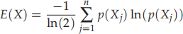
where p(Xj) is the probability value of Xj in the distribution X. For exam-ple, if X = 4, 2, 3, 5, 3, 4, 5, 9, and each element of X can take any values between 0 and 9, then p(X) = 0, 0, 1/8, 2/8, 2/8, 2/8, 0, 0, 0, 1/8.

Write a C function to calculate this entropy of an integer sequence equation, a main function to test your function, and test your function.

Additional

Attempts at these exercises can earn additional marks, but will not count towards the grade of 1–5 for the exercises. Completing all of these exercises does not mean that 6 marks will be obtained—the marks depend on the quality of the answers. It is possible to earn all 6 marks without completing all of these additional exercises.

A4.1 Do the other part (i.e., (a) or (b)) for R6.2. [PDE]

A4.2 Write a C function to calculate the joint entropy of integer sequences X and Y, defined by

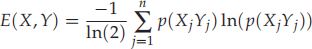
where p(XjYj) is the joint probability of the values Xj and Yj occurring to-gether, i.e., the probability that x = Xj given that y = Yj (which is equal to the probability that y = Yj given that x = Xj ). Write a C function to calculate this entropy, a main function to test your function, and test your function.

A4.3 Find a PDE solver. Discuss the code, if source code is available. Test, and discuss.

A4.4 From computer problems 9.4 in Sauer: Use the Euler-Maruyama method to solve

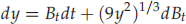
over the interval t = [0, 1] with initial condition y(0) = 0. Note that Bn = ∑i n =0 ∆Bi . Use step sizes of h = 0.1, 0.01, 0.001, and use 5000 simulations for each step size to find the mean value of y(1) and the error. How does the error vary with step size?

A4.5 Implement and test a random number generator.

A4.6 Generate a distribution of random numbers other than uniform or normal. What kind of problem would this distribution be useful for?

A4.7 Find or implement code for high-dimensional optimisation. Test, and dis-cuss.

A4.8 Implement Monte Carlo integration for circles, spheres, etc., using C or some other compiled language. Compare the performance of your code with your Matlab version. Investigate the effect of using single precision instead of double precision.

A4.9 Write a popular science article describing a problem and the use of Monte Carlo methods to solve it.

MODULE 4. HIGH-DIMENSIONAL PROBLEMS 83

Programming hints

Note that rand() and randn() can return a vector or matrix of random numbers. Instead of getting one random number at a time in a loop, you can get them all at once!

• rand(N) and randn(N) will return N × N matrices of random numbers.

• rand(M,N) and randn(M,N) will return M × N matrices of random num-bers.

R4.2 You need to demonstrate a sufficient understanding of the question. This means that you will need to do the integration for multiple dimensions. Going from a 1-sphere (a sphere in 1 dimension) to a 10-sphere is sufficient (That is: 1, 2, 3, 4, 5, 6, 7, 8, 9 and 10).

If you are using rand() in MATLAB or similar, one way to do this is to sam-ple points inside a box. This method is finding the ratio of In/N, where In is how many random points lie inside the sphere, and N is how many points used in the simulation. It is important to note that this is a ratio of the “box” it covers; this means you will need to multiply the ratio by the volume of the box.

Algorithm R4.3 (For a unit sphere).

Draw X from U (0 ,1)

Find the distance the point is from the centre .

Count how many points are inside the sphere .

Calculate ratio = inside / N .

Calculate volume = ratio * boxVolume

R4.3 There are several ways to go about this question. When the walk reaches the top or the bottom of the interval (that is, if at any point the value of the walk equals a or −b) you break the calculation immediately and go to the next calculation. 

The stating point for the walk is 0.

For some, it may be helpful to think of it as a Discrete Markov Chain. Each state is finite, and once it reaches the boundary, it can keep going back to boundary with a probability of 1.

Algorithm R4.3 Easy algorithm, ignoring Murphy’s Law.

Initialse ReachedTheTop

Do N times

Initialise W

* Random walk process *

Stop

* Random Walk process *

while not at the boundary

Draw u from U

if u > q

go up

otherwise

go down

if W is at a

Increment ReachedTheTop

stop

if W is at -b

stop

There is a more advanced algorithm. This is only useful if you are going to vectorise; if you are not going to vectorise, do the one above.

Initialise W

Do M times

Draw dW from sign ( U - q )

W = W + dW

if Wi = a , set Wi to be inf

if Wi = -b , set Wi to be - inf

Stop

Sum up W equal to inf

Question: Why does this algorithm work? Is it mathematically correct?

What does W(W==a) do?

A4.4 Bt is a partial sum, and is related to every random number drawn before (for that walk).

Algorithm R4.4 Non-vectorised.

Calculate the number of steps .

Do N times

* Euler - Maruyama step *

Stop

Find the mean .

* Euler - Maruyama step *

Do number of steps times

Draw Z from N (0 ,1).

Calculate dB and Bt .

Apply Euler - Maruyama scheme

Stop

And of course, a more advanced vectorised version. (Thomas wrote these hints, and he vectorises a lot.)

Draw Z from N (0 ,1)

Calculate Bt and initialise Y

Calculate the number of steps

Do number of steps times

Apply Euler Maruyama - scheme

( using element - wise operations )

Stop

Find the mean .