ECON 483K/556: Advanced Data Analysis Problem Set 2 Fall 2023

Hello, dear friend, you can consult us at any time if you have any questions, add WeChat: daixieit

Fall 2023

ECON 483K/556: Advanced Data Analysis

Problem Set 2

Due Date: November 3, 2023

To receive full mark, you must show your work and submit R script. Your answers should be contained in a single pdf file, separate from the R script that can be used to reproduce your results.

Problem 1

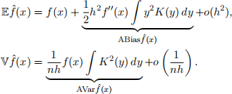
Revisit slide 25 in Lecture 6 Density Estimation. Derive the asymptotic expression for the mean and variance of a kernel density estimator, i.e., show that

Problem 2

Let K : R → R be a kernel function.

(a) Show that a scaled kernel is a density function, i.e., for any h > 0, the function Kh(·) = K(·/h)/h is nonnegative and integrates to one.

(b) Derive the exact expressions for the mean, the second moment, and L 2 -norm of the standar Gaussian and Epanechnikov kernel, i.e., derive

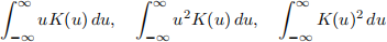
when K is the standard Gaussian and Epanechnikov kernel, respectively.

(c) Let f ˆ denote the kernel density estimator using the Gaussian kernel and let f ˜ denote the one using the Epanechnikov kernel. Suppose the MISE-optimal bandwidth h ∗ is used for each kernel. Compare the relative asymptotic bias and variance of the two kernel density estimators, i.e., compare the ratios

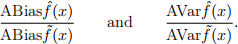
Which one has lower bias? Lower variance?

Problem 3

The leave-one-out cross validation bandwidth matrix Hcv minimizes the criterion function

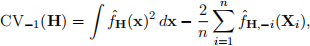
where f ˆH denotes a kernel density estimator using bandwidth matrix H and f ˆH,−i denotes its leave-one-out estimator.

(a) Explain why the average of the leave-one-out estimators is an appropriate way to estimate Ef ˆH(X).

(b) Construct your own R function that computes the diagonal leave-one-out cross-validation bandwidth matrix for a two-dimensional kernel density estimator. Name the function diyH. You may use the kde function in the ks package to construct diyH. The function should also output the bandwidth matrix Hcv that minimizes the criterion function. The function should take as its inputs the data set data (an n × 2 matrix) and two sets of grid points h1 and h2 for the diagonal bandwidth matrix H. The function should output a heat map that shows the value of the criterion function CV−1(h1, h2) for every pair of bandwidths h1 and h2 from the sequences h1 and h2, respectively, that forms a diagonal bandwidth matrix

The function should also output the bandwidth matrix that minimizes the criterion function among all possible pairs of bandwidths from the sequences.

(c) Set the seed number to 1234. Draw 500 observations from the following mixture of bivariate normals:

Name the data set data. Use diyH to compute the diagonal CV bandwidth. In particular, set h1 <- seq(0.01,2,0.01) and h2 <- seq(0.01,2,0.01). What is the value of the bandwidth matrix? Plot the kernel density estimate.

(d) Plot the kernel density estimate using kde and Hlscv.diag in the ks package. Compare the bandwidth matrix you obtained using the ks package and the matrix you obtained using diyH. Plot the kernel density estimate and compare it to the plot you obtained in part (b).

Problem 4

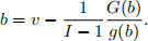
In a first-price sealed-bid auction, each bidder submits a sealed bid, which is not revealed to compet-ing bidders. The bidder who submits the highest bid wins the auction and pays the price equivalent to the submitted bid. Because bidders aim to maximize expected returns, the bids they submit may differ from their valuations—their willingness to pay for the item being auctioned. Under certain microeconomic assumptions, it can be shown that if a bidder’s valuation for the item is v, then the bid b she submits is given by

where H(b) is the probability of winning the auction with bid amount b and h(b) its derivative. If there are I bidders, G denotes the distribution of all bids and g its density, then it can be shown that

Suppose one has data set on I bids across n auctions. One way to estimate the density of valuations is by estimating the kernel density of pseudo-valuations, i.e., estimate the density using pseudo-valuations

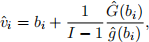
is the empirical c.d.f. estimated using I × n bids and gˆ is the kernel density estimate of g. This is a simplified description of Guerre, Perrigne and Vuong’s “Optimal nonparametric estimation of first-price auctions,” Econometrica, Vol. 68, No. 3, 2000, pp. 525–574. Reading the article may help answer some of the questions below.

(a) Download auctions.Rdata from Brightspace. Each column of the file is a simulated data set of 400 auctions with two bidders. There are 999 simulated data sets in the file. Use column 1 to estimate the the density of bidder valuations. When estimating the kernel density, use the kde function and hpi bandwidth selection in ks package. Plot the density estimate.

(b) Overlay the density of a Beta(2, 2) distribution on the plot obtained in part (a). This is the true density of valuations. Are they similar?

(c) Use the remaining columns to obtain 998 kernel density estimates for valuations. For each v = 0, 0.01, 0.02, . . . , 0.98, 0.99, 1, compute the average of the density estimates f ˆ(v). Plot the averages along with the true density. Compare the two curves and discuss whether the similarity or differences across different values of v is expected based on what you learned in class. Why or why not would the result differ from your expectations?

(d) For each v = 0, 0.01, 0.02, . . . , 0.98, 0.99, 1, calculate the 5th and 95th percentiles of density estimates f ˆ(v). Plot the lower and upper percentile band on the same graph. Compare the band to the true density. Discuss whether the shape of the band is expected based on what you learned in class.