ETX2250/ETF5922: Data Visualization and Analytics

Coding questions

For the coding part of questions, you are required to write the necessary R code and input the R code into the answer box for each question (similar to Assignment 1). Code should be written in "tidyverse" style -- with the functions learned from the lectures and pipes to join commands. Assume the following libraries have been loaded into R for you when typing   your R code in the answer boxes:

library(tidyverse)

library(ggplot2)

library(here)

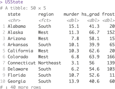
Data background: For questions 1 - 4, we will use the data containing some information for the states of the United States in 1977. In particular, we have the murder rates, percentage of highschool graduates, and percentage of frost.  Recall that we have seen this data set in the tutorials, and this is a modified version of the data set. Assume the data is already read into R and saved as `USState` with 50 rows and 6 variables. Each row represents a different state.

The first column is the state, the second is the region the state belongs to and the remaining column measures the characteristics of the state. The first ten rows of `USState` look like this:

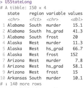
1)  Suppose we want our data frame to be in a ‘long’ format sowe can plot them easily.

Please write the necessary R code to change the data set `USState` into a long format   and store the resulting data object as `USStateLong` (Hint: you could use murder:frost to select columns from `murder` to `frost`). Input your R code into the provided answer box. The resulting data frame should look like the one below.

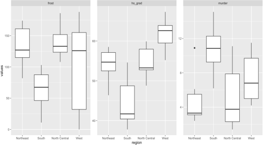
2)  Using the data stored in `USStateLong`, write R code to make a boxplot for the

variables region on the x-axis, and the values of the different variables on they-axis., and facet by variable (Hint: use scales=”free_y” in the facet_wrap function to replicate the plot). The resulting plot should look like the one below:

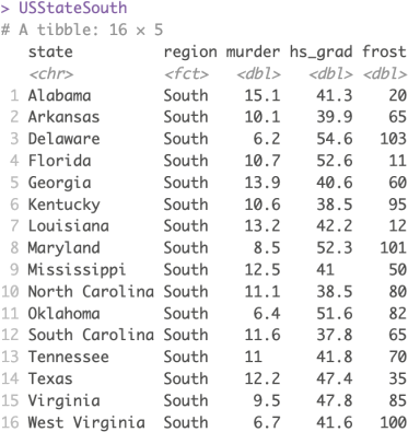
3)  Suppose now we want to focus on the southern states only. Write R code to keep the observations for the region equal to South and save the new data frame in a data object called `USStateSouth`.  The resulting data frame should look like the one below:

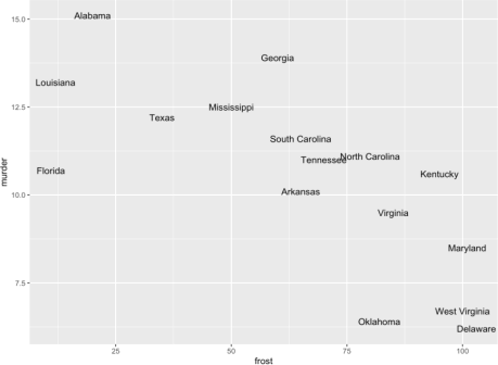
4)  Using the data stored in `USStateSouth`, write R code to make a text plot for the variables frost on the x-axis, and the murder on they-axis and using state as the text labels.  The resulting plot should look like the one below:

Concept questions

1. Compare and contrast regression and classification.

2. What are the limitations of hierarchical clustering?

3. What is the difference between single linkage and complete linkage?

4. Describe an ROC (receiver operating characteristic curve). What does it plot and what is it used for?

Computation questions

1. After the first stage of the kmeans clustering algorithm with two variables (x andy), we have three centroids represented by (we have named them for convenience):

We have an observation (x1=12, x2=40). Using Euclidean distance and Manhattan distance, calculate which cluster the point belongs to and report this distance. Round to two decimal   places.

2. Calculate the root mean square error for the predicted and true values observed in the table below. Round to two decimal places.

3. For the following table of predicted default vs. whether the individual actually defaulted (positive), what are themisclassification errors for both prediction methods?

4. An online provider of statistics courses is interested in assessing alternative sequencing and combinations of courses and therefore wishes to conduct association analysis on its data for past students. In the table, each row represents an individual student and each column represents a statistics course that they offer as identified by the column headings.