STAT3405: Introduction to Bayesian Computing and Statistics Computer Lab Problems #3

Important:  This assignment is assessed.  Your work for this task must be submitted by 11:00pm  on Friday, 22 September 2023.

Your solution should be submitted via LMS.

The expectation for a submission are:

•  The questions are answered in complete sentences.  Click on “Create Submission” on LMS’ assign- ment submission page and enter your answers into the window that opens. Marks will be awarded for

- the correctness of the answers and that they are given in complete sentences,

- the conciseness of the answers; and

- the answers being software agnostic and not referring to any code that you may have used to find them.

•  That numerical answers are rounded to an appropriate number of digits.

•  Code  used to  answer the questions was saved into a plain text file1 and  then  attached  to the submission (see “Attach Files”), so that it will be easy to re-run the code and check it.  Code should be in Stan or BUGS. Please do not attach Word documents, PDF, or other binary formats, the only exceptions are (a) files produced from R notebooks as long as the original R notebook is attached too and (b) files saved in OpenBUGS’ *.odc format but even that format should be avoided

if the file only contains BUGS code.

Marks will be awarded for

- the correctness of the code, i.e. how easy it is to read it2 ; and

- how easy it is to get the code to run, if necessary.

You may receive comments on the efficiency of your code, but there are no marks for efficiency.

Unless special consideration is granted, any student failing to submit work by the deadline will receive a penalty for late submission (as described in the unit outline).

Plagiarism:  You are encouraged to discuss assignments with other students and to solve problems together. However, the work that you submit must be your sole effort (i.e. not copied from anyone else). If you are found guilty of plagiarism you may be penalised.  You are reminded of the University’s policy on ‘Academic Conduct’ and ‘Academic Misconduct’ (including plagiarism):

http://www.student.uwa.edu.au/learning/resources/ace/conduct

Various material at the following URL might be helpful too:

https://www.uwa.edu.au/students/study-success/studysmarter

Let us revisit the example from second example in today’s computer lab.  First read in the data, replacing “PATH_TO_DATA” with the appropriate path

dat <- read.csv("PATH_TO_DATA/rats-ctt.csv")

Next we store the first column again into the object x and the remaining columns in the object y, turning it from a object of class data.frame into an object of class matrix at the same time:

x <- 0:4

y <- data.matrix(dat[, -(1:2)])

As the object y is a matrix, we can use the command matplot() to plot the data:

matplot(x, t(y), col = "black", pch = 20)

It looks plausible that the mean weight increases linearly with time (week), but we can clearly see that we have an issue with responses showing less variability early on and more variability in the later weeks. In other words, we have a problem with heteroscedasticity, i.e. the assumption of equal variance underlying the simple linear regression model is questionable.

The  R  package matrixStats (which you might have to install first) allows us to easily calculate the (sample) standard deviations3 of the 48 observations that we have for each week:

library(matrixStats)

(SDs <- colSds(y))

##     Week0     Week1     Week2     Week3     Week4

##  4.506406  8.052711 10.517114 16.822604 23.924799

We see that the sample standard deviations clearly increase over the weeks.

This confirms that we should model the Yij  as:

Yij|µj, σj(2) ∼ N (µj, σj(2)),        i = 1, . . . , 27,    j = 1, . . . , 5

where we model the means as µj  = α+βxj , j = 1, . . . , 5. But how should we model the σj(2)s or, equivalently,

the σjs?  Note that the sample standard deviations that we just calculated are, of course, estimates for the σjs.

One possibility would be to model the σjs as (would we need to impose any constraints on γ0  and/or γ1 ?):

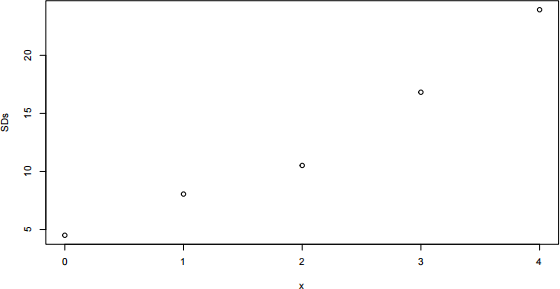
σj  = g(xj|γ0 , γ1 ) = γ0 + γ1 xj,    j = 1, . . . , 5                                                  (1)

If this model is appropriate, then the sample standard deviations should increase linearly with time, i.e. we would expect the points in the following plot to fall more or less onto a straight line:

plot(x, SDs)

Another  possibility would  be to  model the  σis  as  (would  we  need  to  impose  any  constraints  on  γ0 and/or γ1 ?):

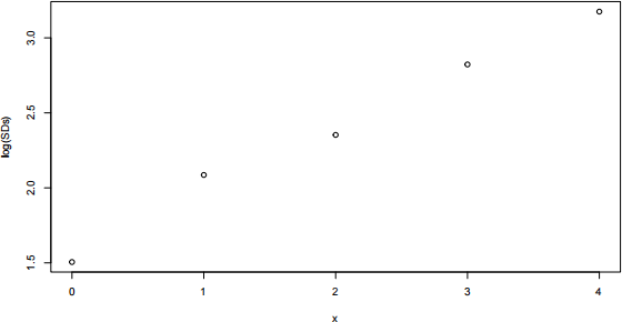
σj  = g(xj|γ0 , γ1 ) = exp (γ0 + γ1 xj) ,    j = 1, . . . , 5                                            (2)

If this model is appropriate, then the log of the sample standard deviations should increase linearly with time, i.e. we would expect the points in the following plot to fall more or less onto a straight line:

plot(x, log(SDs))

Yet another possibility would be to model the σis as (would we need to impose any constraints on γ0 and/or γ1 ?):

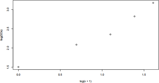
σj  = g(xj|γ0 , γ1 ) = γ0 (xj  + 1)γ1 ,    j = 1, . . . , 5                                                (3)

If this model is appropriate, then the log of the sample standard deviations should increase linearly with the logarithm of time, i.e. we would expect the points in the following plot to fall more or less onto a straight line:

plot(log(x + 1), log(SDs))